Mechatronic Systems Programming in C++
Copyright © 2014 Péter Tamás Phd, Antal Huba Phd, József Gräff

A tananyag a TÁMOP-4.1.2.A/1-11/1-2011-0042 azonosító számú „ Mechatronikai mérnök MSc tananyagfejlesztés ” projekt keretében készült. A tananyagfejlesztés az Európai Unió támogatásával és az Európai Szociális Alap társfinanszírozásával valósult meg.

Manuscript completed: February 2014
Language reviewed by: Ágoston Nagy
Published by: BME MOGI
Editor by: BME MOGI
2014
- I. Basics and data management of C++
- I.1. Creation of C++ programs
- I.2. Basic data types, variables and constants
- I.3. Basic operations and expressions
- I.4. Control program structures
- I.5. Exception handling
- I.6. Pointers, references and dynamic memory management
- I.7. Arrays and strings
- I.8. User-defined data types
- II. Modular programming in C++
- II.1. The basics of functions
- II.1.1. Defining, calling and declaring functions
- II.1.2. The return value of functions
- II.1.3. Parametrizing functions
- II.1.3.1. Parameter passing methods
- II.1.3.2. Using parameters of different types
- II.1.3.2.1. Arithmetic type parameters
- II.1.3.2.2. User-defined type parameters
- II.1.3.2.3. Passing arrays to functions
- II.1.3.2.4. String arguments
- II.1.3.2.5. Functions as arguments
- II.1.3.2.6. Default arguments
- II.1.3.2.7. Variable length argument list
- II.1.3.2.8. Parameters and return value of the main() function
- II.1.4. Programming with functions
- II.2. How to use functions on a more professional level?
- II.3. Namespaces and storage classes
- II.3.1. Storage classes of variables
- II.3.2. Storage classes of functions
- II.3.3. Modular programs in C++
- II.3.4. Namespaces
- II.4. Preprocessor directives of C++
- III. Object-oriented programming in C++
- III.1. Introduction to the object-oriented world
- III.2. Classes and objects
- III.3. Inheritance (derivation)
- III.4. Polymorphism
- III.5. Class templates
- III.5.1. A step-be-step tutorial for creating and using class templates
- III.5.2. Defining a generic class
- III.5.3. Instantiation and specialisation
- III.5.4. Value parameters and default template parameters
- III.5.5. The "friends" and static data members of a class template
- III.5.6. The Standard Template Library (STL) of C++
- IV. Programming Microsoft Windows in C++
- IV.1. Specialties of CLI, standard C++ and C++/CLI
- IV.1.1. Compiling and running native code under Windows
- IV.1.2. Problems during developing and using programs in native code
- IV.1.3. Platform independence
- IV.1.4. Running MSIL code
- IV.1.5. Integrated development environment
- IV.1.6. Controllers, visual programming
- IV.1.7. The .NET framework
- IV.1.8. C#
- IV.1.9. Extension of C++ to CLI
- IV.1.10. Extended data types of C++/CLI
- IV.1.11. The predefined reference class: String
- IV.1.12. The System::Convert static class
- IV.1.13. The reference class of the array implemented with the CLI array template
- IV.1.14. C++/CLI: Practical realization in e.g. in the Visual Studio 2008
- IV.1.15. The Intellisense embedded help
- IV.1.16. Setting the type of a CLR program.
- IV.2. The window model and the basic controls
- IV.2.1. The Form basic controller
- IV.2.2. Often used properties of the Form control
- IV.2.3. Events of the Form control
- IV.2.4. Updating the status of controls
- IV.2.5. Basic controls: Label control
- IV.2.6. Basic controls: TextBox control
- IV.2.7. Basic controls: Button control
- IV.2.8. Controls used for logical values: CheckBox
- IV.2.9. Controls used for logical values: RadioButton
- IV.2.10. Container object control: GroupBox
- IV.2.11. Controls inputting discrete values: HscrollBar and VscrollBar
- IV.2.12. Control inputting integer numbers: NumericUpDown
- IV.2.13. Controls with the ability to choose from several objects: ListBox and ComboBox
- IV.2.14. Control showing the status of progressing: ProgressBar
- IV.2.15. Control with the ability to visualize PixelGrapic images: PictureBox
- IV.2.16. Menu bar at the top of our window: MenuStrip control
- IV.2.17. The ContextMenuStrip control which is invisible in basic mode
- IV.2.18. The menu bar of the toolkit: the control ToolStrip
- IV.2.19. The status bar appearing at the bottom of the window, the StatusStrip control
- IV.2.20. Dialog windows helping file usage: OpenFileDialog, SaveFileDialog and FolderBrowserDialog
- IV.2.21. The predefined message window: MessageBox
- IV.2.22. Control used for timing: Timer
- IV.2.23. SerialPort
- IV.3. Text and binary files, data streams
- IV.3.1. Preparing to handling files
- IV.3.2. Methods of the File static class
- IV.3.3. The FileStream reference class
- IV.3.4. The BinaryReader reference class
- IV.3.5. The BinaryWriter reference class
- IV.3.6. Processing text files: the StreamReader and StreamWriter reference classes
- IV.3.7. The MemoryStream reference class
- IV.4. The GDI+
- IV.4.1. The usage of GDI+
- IV.4.2. Drawing features of GDI
- IV.4.3. The Graphics class
- IV.4.4. Coordinate systems
- IV.4.5. Coordinate transformation
- IV.4.6. Color handling of GDI+ (Color)
- IV.4.7. Geometric data (Point, Size, Rectangle, GraphicsPath)
- IV.4.8. Regions
- IV.4.9. Image handling (Image, Bitmap, MetaFile, Icon)
- IV.4.10. Brushes
- IV.4.11. Pens
- IV.4.12. Font, FontFamily
- IV.4.13. Drawing routines
- IV.4.14. Printing
- References:
- V. Developing open-source systems
- VI. Aim-specific applications
- A. Appendix – Standard C++ summary tables
- A.1. ASCII code table
- A.2. Reserved keywords in C++
- A.3. Escape characters
- A.4. C++ data types and their range of values
- A.5. Statements in C++
- A.6. C++ preprocessor directives
- A.7. Precedence and associativity of C++ operations
- A.8. Some frequently used mathematical functions
- A.9. C++ storage classes
- A.10. Input/Output (I/O) manipulators
- A.11. The standard C++ library header files
- B. Appendix – C++/CLI summary tables
- I.1. Project selection
- I.2. Project settings
- I.3. Possible source files
- I.4. Window of the running program
- I.5. Steps of C++ program compilation
- I.6. Classification of C++ data types
- I.7. Functioning of a simple if statement
- I.8. Logical representation of if-else structures
- I.9. Logical representation of multi-way branches
- I.10. Logical representation of while loops
- I.11. Logical representation of for loops
- I.12. Logical representation of do-while loops
- I.13. C++ program memory usage
- I.14. Dynamic memory allocation
- I.15. Graphical representation of an one-dimensional array
- I.16. Graphical representation of a two-dimensional array
- I.17. The relationship between pointers and arrays
- I.18. Two-dimensional arrays in memory
- I.19. Dynamically allocated row vectors
- I.20. Dynamically allocated pointer vector and row vectors
- I.21. String constant in memory
- I.22. String array stored in a two-dimensional array
- I.23. Optimally stored string array
- I.24. Structure in memory
- I.25. Processing data in the program CDCatalogue
- I.26. A singly linked list
- I.27. Union in memory
- I.28. The layout of the structure date in memory
- II.1. Function definition
- II.2. Steps of calling a function
- II.3. Graph of the third degree polynomial
- II.4. The interpretation of the parameter argv
- II.5. Providing command line arguments
- II.6. Calculating the area of a triangle
- II.7. Variable scopes
- II.8. The compilation process in C++
- III.1. The object myCar (an instance of the class Truck)
- III.2. Inheritance
- III.3. Multiple inheritance
- III.4. The class Employee and its objects
- III.5. The multiple inheritance of I/O classes in C++
- III.6. Hierarchy of geometrical classes
- III.7. Using virtual base classes
- III.8. Early binding example
- III.9. Late binding example
- III.10. Virtual method tables of the example code
- IV.1. The memory before cleaning
- IV.2. The memory after cleaning
- IV.3. The window in the View/Designer
- IV.4. The program in the View/Code window
- IV.5. The Toolbox
- IV.6. The Control menu
- IV.7. The Properties Window
- IV.8. The Event handlers
- IV.9. A defined Event Handler
- IV.10. The Intellisense window
- IV.11. Solution Explorer menu
- IV.12. Project properties
- IV.13. Part of the program’s window
- IV.14. Normal size picturebox on the form
- IV.15. Stretched size picturebox on the form
- IV.16. Automatic sized picturebox on the form
- IV.17. Centered image in the picturebox on the form
- IV.18. Zoomed bitmap in the picturebox on the form
- IV.19. Menustrip
- IV.20. Menuitem on the menustrip
- IV.21. The Help menu
- IV.22. The submenu
- IV.23. The contextmenu
- IV.24. Toolkit on toolstrip
- IV.25. The MessageBox
- IV.26. Binary file processing
- IV.27. The classes of GDI+
- IV.28. The drawn line automatically appears after every resizing activity.
- IV.29. If we do not draw in Paint then the blue line disappears when maximizing after minimizing.
- IV.30. General axonometry
- IV.31. Isometric axonometry
- IV.32. Military axonometry
- IV.33. The default coordinate-system on form
- IV.34. Cube in axonometry
- IV.35. Central projection
- IV.36. The perspective views of the cube
- IV.37. Setting the distortion
- IV.38. The distortion
- IV.39. Trasnlating and scaling with a matrix
- IV.40. Translation and rotation
- IV.41. Trasnlating and shearing
- IV.42. The mm scale and the PageScale property
- IV.43. Color mixer
- IV.44. Alternate and Winding curve chains
- IV.45. Elliptical arc
- IV.46. Cubic Bezier curve
- IV.47. Cubic Bezier curve joined continously
- IV.48. The cardinal spline
- IV.49. Catmull-Rom spline
- IV.50. Text in the figure
- IV.51. Two concatenated figures connected and disconnected
- IV.52. Widened figure
- IV.53. Distorted shape
- IV.54. Clipped figure
- IV.55. Vectorial A
- IV.56. Rasterized A
- IV.57. Image on the form
- IV.58. Halftone representation
- IV.59. Rotated image
- IV.60. Coloring bitmap
- IV.61. Non-managed bitmap manipulating
- IV.62. Brushes
- IV.63. Pens
- IV.64. Character features
- IV.65. Traditional character widths
- IV.66. ABC character widths
- IV.67. Font families
- IV.68. Font distortions
- IV.69. Zoomed image and distorted zoomed image
- IV.70. The OneNote program is the default printer
- VI.1. The block diagram of PIC32MX
- VI.2. Possibilities of connecting a RealTek SOC
- VI.3. The example program
- VI.4. The MPLAB IDE
- VI.5. The structure of CORBA
- VI.6. The structure of ICE programs
- VI.7. The ICE libraries
Chapter I. Basics and data management of C++
- I.1. Creation of C++ programs
- I.2. Basic data types, variables and constants
- I.3. Basic operations and expressions
- I.4. Control program structures
- I.5. Exception handling
- I.6. Pointers, references and dynamic memory management
- I.7. Arrays and strings
- I.8. User-defined data types
Knowledge necessary for program development in language C++ is detailed divided into three large categories. Category one (Chapter I, Basics and data management of C++ ) presents basic elements and program structures most of which can be found both in language C and C++. A program containing one single main() function is enough to practice the curriculum.
The next chapter (Chapter II, Modular programming in C++) assists in creating well-structured C and C++ programs according to algorithmic thinking using the presented solutions. Functions play the main role in this part.
The third chapter (Chapter III, Object-oriented programming in C++) presents the means of the nowadays more and more dominant object-oriented program building. Here classes that encapsulate data and the operations to be carried out on them into one single unit are in focus.
I.1. Creation of C++ programs
Before the elements of language C++ are detailed, issues on the creation and running of C++ programs are to be overviewed. A few rules that are to be applied when writing C++ source codes, program structures and steps needed for running in Microsoft Visual C++ system are described.
I.1.1. Some important rules
Standard C++ language belongs to conventional programming languages in case of which the creation of the program involves typing the whole text of the program, as well. When typing the text (source code) of the program a few restrictions have to be considered:
The basic elements of the program can only contain the characters of the 7 bit ASCII code table (see in Appendix Section A.1, “ASCII code table”), however character and text constants, as well as remarks may contain characters of any coding (ANSI, UTF-8, Unicode). A few examples:
/* Value is given for an integer, a character and a text
  (string)  variable (multiline remark) */
int variable = 12.23;  // value giving (remark until the
                       // end of the line)
char sign = 'Á';
string header  = "Programming is fun"
C++ compiler differentiates small and capital letters in the words (names) used in the program. Most of names that make up the language contain only small letters.
Certain (English) words cannot be used as own names since these are keywords of the compiler (see in Appendix Section A.2, “Reserved keywords in C++”).
In case of creating own names please note that they have to start with a letter (or underscore sign), and should contain letters, numbers or underscore signs in their other positions. (Please note that it is not recommended to use the underscore sign.)
One last rule before writing the first C++ program is that we should not too long however so called talkative names define such as: ElementSum, measurementlimit, piece, RootFinder.
I.1.2. The first C++ program in two versions
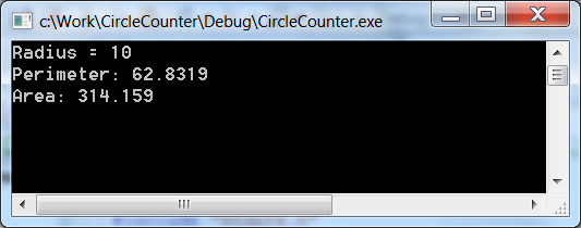
Since language C++ is compatible from the top with the standard (1995) C language, in case of creating simple programs C programming knowledge can also result in success. Let’s take the example of perimeter and area calculation of a circle in plane. The algorithm is very simple, since after the radius is entered, only a few formulas have to be calculated.
The two solutions below only differ from each other in the input/output operations basically. In style C case printf() and scanf() functions are used, while in the second C++ type case objects cout and cin are applied. (In case of further examples the latter solution is used.) The source code has to be placed into a .CPP extension text file in both cases.
Style C solution with a slight modification can also be compiled with a C compiler:
// Circle1.cpp
#include "cstdio"
#include "cmath"
using namespace std;

int main()
{
    const double pi = 3.14159265359;
    double radius, area, perimeter;
    // Reading radius
    printf("Radius = ");
    scanf("%lf", &radius);
    // Calculations
    perimeter = 2*radius*pi;
    area = pow(radius,2)*pi;
    printf("Perimeter: %7.3f\n", perimeter);
    printf("Area: %7.3f\n", area);
    // Waiting for pressing Enter
    getchar();
getchar();
    return 0;
}
The solution that uses C++ objects is a little easier to understand:
// Circle2.cpp
#include "iostream"
#include "cmath"
using namespace std;

int main()
{
    const double pi = 3.14159265359;
    // Reading radius
    double radius;
    cout << "Radius = ";
    cin >> radius;
    // Calculations
    double perimeter = 2*radius*pi;
    double area = pow(radius,2)*pi;
    cout << "Perimeter: " << perimeter << endl;
    cout << "Area: " << area << endl;
    // Waiting for pressing Enter
    cin.get();
    cin.get();
    return 0;
}
Both solutions use C++ and own names as well (radius, area, perimeter, pi). It is an essential rule that all names have to be declared for the C++ compiler before first usage. In the example lines that start with double and constdouble not only declare the names but also create (define) their related storages in the memory. However, similar descriptions are not found for names printf(), scanf(), pow(), cin and cout. The declarations of these names can be found in the (#include) files (cstdio, cmath and iostream, respectively) included at the beginning of the program. The names are closed in the namespace std.
Function printf() presents data in a formatted way. If data are directed (<<) to object cout, formatting is more complicated, but in that case format elements belonging to different data types does not have to be dealt with. The same is true for scanf() and cin elements used for data entry. Another important difference is the security of the applied solution. In case scanf() is called, the beginning address (&) of the memory space for data storage has to be entered, and this way several errors may arise in the program. Oppositely, application of cin is completely safe.
Another remark to getchar() and cin.get() calls at the end of programs. After the last call of scanf() and cin the data entry buffer maintains data correspondent to key Enter. Since both functions that read characters carry out processing after key Enter is pressed, the first calls only remove Enter that remained in the buffer, and only the second call is waiting for another Enter pressing.
In both cases an integer (int) type function, named main() , contains the main part of the program, closed between the curly brackets that include body the of the function. Functions – as in mathematics – have values that are defined after statement return in language C++. The explanation of values comes from the ancient versions of language C, and accordingly 0 means that everything was all right. In case of main() this function value is received by the operation system since, which calls the function as well (starts the program running this way).
I.1.3. Compilation and running of C++ programs
In most development systems the basis of program creation is the generation of a so called project. Firstly, the type of the application has to be chosen, and then the source files have to be added to the project. From the several possibilities offered by system Visual C++ the Win32 console application is the simple C++ application type with text interface. Let’s see the necessary steps!
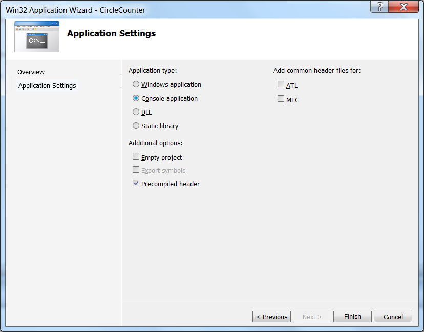
After selections File / New / Project… Win32 / Win32 Console Application the name of the project has to be entered:
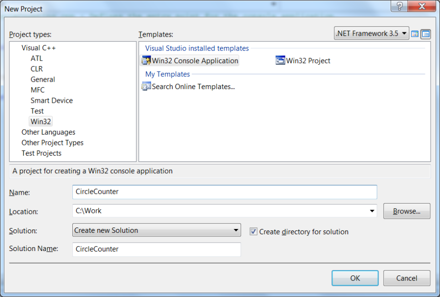
After key OK is pressed, the Console application wizard starts, and using its settings an empty project can be created:
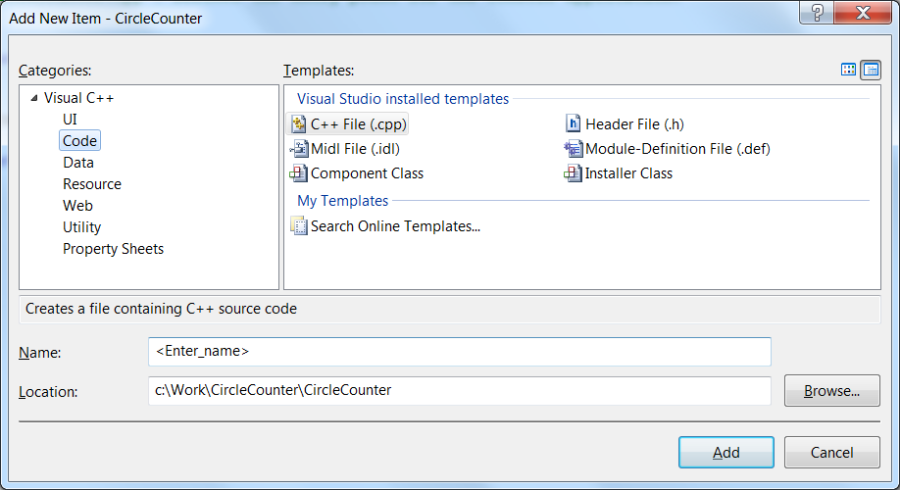
After pressing key Finish the solution window (Solution Explorer) appears, where a new source can be added to the project ( Add / New Item… ) using mouse right click on Source Files .
After the text of the program is typed, compilation can done through menu points Build / Build Solution or Build / Rebuild Solution . In case of successful compilation (CircleCalculation - 0 error(s), 0 warning(s)) the program can be started by choosing menuitem Debug / Start Debugging (F5) or Debug / Start Without Debugging (Ctrl+F5).
After menu Build / Configuration Manager... is selected a window pops up where either the debug ( Debug ) or final ( Release ) version can be chosen to be compiled. (This selection determines the content of the file to be run and its place on the disk.)
In case of any Build , compilation is carried out in several steps. Figure I.5, “Steps of C++ program compilation” shows these steps.
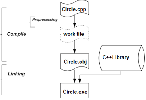
The preprocessor interprets lines starting with hash mark sign (#) and as a result source code in language C++ is created. C++ compiler compiles this code to an object code that misses the machine code that realizes library elements. As the last step the linker fills this gap and transforms the complete machine (native) code to an executable application.
It is to be noted that in case of projects that contain more source files (modules) preprocessor and compiler carry out compilation module by module and the object modules created this way are built together into one single executable file by the linker.
After running the program has to be saved so that we can work with it later. There are several possible solutions, however the next, already proven steps can help us: first all files are saved onto the disk ( File / SaveAll ), then the project is closed together with the solution ( File / Close Solution ). (Solution denotes the set of linked projects that can be recompiled in one single step if necessary.)
Finally let’s take a look at the directory structure that is created on the hard disk when the project is compiled.
C:\Work\CircleCalculation\CircleCalculation.sln
C:\Work\CircleCalculation\CircleCalculation.ncb
C:\Work\CircleCalculation\Debug\CircleCalculation.exe
C:\Work\CircleCalculation\Release\CircleCalculation.exe
C:\Work\CircleCalculation\CircleCalculation\CircleCalculation.vcproj
C:\Work\CircleCalculation\CircleCalculation\Circle1.cpp
C:\Work\CircleCalculation\CircleCalculation\Debug\Circle1.obj
C:\Work\CircleCalculation\CircleCalculation\Release\ Circle1.obj
Debug and Release directories that can be found above this level contain the executable application, while directories below with the same names contain work files. These four folders can be deleted since they will be created again during compilation. It is also recommended to delete file Circle calculation.ncb that assists the intellisense services of development environment since its size can be quite large. The solution (project) can be reopened with the Circle calculation.sln file ( File / Open / Project / Solution ).
I.1.4. Structure of C++ programs
As the previous part revealed, all programs written in language C++ can be found in one or more source files (compilation unit, module), the extension of which is .CPP. C++ modules can be compiled to object codes independently.
So called declaration (include, header) files usually belong to the program as well and they can be integrated in the source files using precompilation statement #include. Include files cannot be compiled independently, however most development environments support their precompilation, accelerating the processing of C++ modules this way.
The structure of C++ modules follows that of C language programs. The program code – according to the principle of procedural programming – is placed in functions. Data (declarations/definitions) can be found both outside (globally, at file level) and within (on local level) the functions. The former are called external (extern) while the latter are classified in the automatic (auto) storage class by the compiler. The example program below illustrates this:
// C++ preprocessor directives
#include <iostream>
#define MAX 2012

// in order to reach the standard library names
using namespace std;

// global declarations and definitions
double fv1(int, long);            // function prototype
const double pi = 3.14159265;     // definition

// the main() function
int main()
{
   /* local declarations and definitions
      statements                               */
   return 0;  // exit the program
}
// function definition
double fv1(int a, long b)
{
   /* local declarations and definitions
      statements                               */
   return a+b; // return from the functions
}
In language C++ object-oriented (OO) approach may also be used when creating programs. According to this principle, the basic unit of our program is the class that encapsulates functions and data definitions (for details see Chapter III, Object-oriented programming in C++). In this case function main() defines the entry point of our program. Classes are usually placed between global declarations, either directly in the C++ module or by the including of a declaration file. „Knowledge” placed in a class can be reached through the instances (variables) of the class.
Let’s take the example of circle calculation task defined with object-oriented approach.
/// Circle3.cpp
#include "iostream"
#include "cmath"
using namespace std;

// Class definition
class Circle
{
        double radius;
        static const double pi;
    public:
        Circle(double r) { radius = r; }
        double Perimeter() { return 2*radius*pi; }
        double Area() { return pow(radius,2)*pi; }
};
const double Circle::pi = 3.14159265359;

int main()
{
    // Reading radius
    double radius;
    cout << "Radius = ";
    cin >> radius;
    // Creation and usage of object Circle
    Circle circle(radius);
    cout << "Perimeter: " << circle.Perimeter() << endl;
    cout << "Area: " << circle.Area() << endl;
    // Waiting for pressing Enter
    cin.get();
    cin.get();
    return 0;
}
I.2. Basic data types, variables and constants
When programming, we attempt to make our activities comprehensible for computers in order that they could help us do those tasks or that they do those tasks for us. When we work, we receive data that we store in general to process them and to extract information from them later. Data are really diverse but most of them consist of numbers or texts in everyday life.
In this chapter, we deal with describing and storing data in C++. We also learn how to receive data (from an input) and how to visualize them.
On the basis of the Neumann principle, data are stored in a uniform way in computer memory, that is why programmers have to provide the type and the features of the data in a C++ program.
I.2.1. Classification of C++ data types
The data type determines the number of bits they occupy in memory and their interpretation (variable). It also affects the way data are processed since C++ is a strongly typed language, therefore compilers check many things.
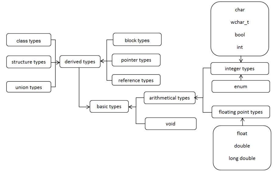
C++ data types (shortened as types) can be classified in several ways. Let's use the classification of Microsoft VC++ language (Figure I.6, “Classification of C++ data types”). According to it, there are basic data types that can store one value (integer, character, real number). However, there are also derived data types that are based on basic types, but they allow the creation of data structures that may store more values.
I.2.1.1. Type modifiers
In C++ language the meaning of basic integer types can be altered by type modifiers . The signed/unsigned modifier pair determines whether the stored bits can be interpreted as negative numbers or not. With the short/long pair size of the storage can be fixed to 16 or 32 bits. Most C++ compilers support 64 bits storage with the long long modifier, therefore it will also be dealt with in this book. Type modifiers can also be used as type definitions alone. Possible type modifiers are summarized in the following table. Elements in each row designate the same data type.
|
char |
signed char | ||
|
short int |
short |
signed short int |
signed short |
|
int |
signed |
signed int | |
|
long int |
long |
signed long int |
signed long |
|
long long int |
long long |
signed long long int |
signed long long |
|
unsigned char | |||
|
unsigned short int |
unsigned short | ||
|
unsigned int |
unsigned | ||
|
unsigned long int |
unsigned long | ||
|
unsigned long long int |
unsigned long long |
The required memory of arithmetical types with type modifiers and the value range of stored data are summarized in Appendix Section A.4, “C++ data types and their range of values”.
Basic types are detailed in the present subchapter, while derived types are treated in the following parts of Chapter I, Basics and data management of C++ .
I.2.2. Defining variables
Storing data in memory and accessing them is vital for every C++ computer program. That is why, we start with getting to know memory spaces to which names are assigned, i.e. variables. In most cases, variables are defined, i.e. their type is provided (they are declared), and memory space is allocated for them. (In the beginning, we rely on compilers for memory allocation.)
The total definition row of a variable is very complex at first sight; however, it is done in a much simpler way in practice.
〈storage class〉 〈type qualifier〉 〈type modifier ... 〉 typevariable name 〈= initial value〉 〈, … 〉;
〈storage class〉 〈type qualifier〉 〈type modifier ... 〉 typevariable name 〈(initial value〉 〈, … 〉;
(In the previous generalized forms, the 〈 〉 signs indicate optional elements while the three points show that a definition element can be repeated.)
The storage classes – auto, register, staticand extern – of C++ determine the lifetime and visibility of variables. At first, storage classes are not defined explicitly, therefore the default case of C++ is used, in which variables defined outside functions have extern (global), while variables defined within a function have auto (local) storage classes. Extern variables are created when the program is started, exist until its end and can be accessed from anywhere during execution. On the contrary, auto variables are born when a function is entered and they are deleted when the function is exited. Therefore they can be accessed within the function.
With type qualifiers further information can be assigned to variables.
Variables with const keyword cannot be modified (they are read-only, i.e. constants).
The volatile type qualifier indicates that the value of the variable can be modified by a code independent of our program (e.g. by another running process or thread). The word volatile tells the compiler that it is not known in advance what will happen to that variable. (That is why, compilers get the value of the variable from the memory each time a volatile variable is referenced.)
int const
const double
volatile char
float volatile
const volatile bool
I.2.2.1. Initial values of variables
Variable definition ends with giving an initial value. Initial values can be provided after an equal sign or between parentheses:
using namespace std;

int sum, product(1);

int main()
{
    int a, b=2012, c(2004);
    double d=12.23, e(b);
}
In this example, there is no initial value for two variables (sum and a), which leads in general to a program error. However, the variable sum has the initial value of 0, since global variables are always initialized (to zero) by compilers. But the local a is a different case since its initial value is provided by the actual content of the memory allocated for the variable and that can be anything. In these cases, the value of these variables can be set by assignment before their usage. During assignment, the value of the expression on the right of the equal sign is assigned to the variable on the left:
a = 1004;
In C++ language the initial values can be provided by any compile-time and run-time expressions.:
#include <cmath>
#include <cstdlib>
using namespace std;

double pi = 4.0*atan(1.0);   // π
int randomnumber(rand() % 1000);

int main()
{
    double alimit = sin(pi/2);
}
It is important that definition and value assignment statements end with a semicolon.
I.2.3. Basic data types
Basic data types are the equivalents of digits or letters in human language. A PhD dissertation in Mathematics or Winnie the Pooh can be created with the help of them. In the following overview, integer types are divided into smaller groups.
I.2.3.1. Character types
The char type has a double role. On one hand, it makes it possible to store ASCII (American Standard Code for Information Interchange) characters (Appendix Section A.1, “ASCII code table”), on the other hand, it can be used as one byte signed integer.
char lettera = 'A';
cout << lettera << endl;
char response;
cout << "Yes or No? ";
cin>>response;
// or
response = cin.get();
The double nature of char type is well represented by the possibilities how constant values (literals) can be assigned to them. Characters can be provided between apostrophes or by their integer code. Besides decimal numbers, character codes can be given in octal format (starting with zero) or in a hexadecimal format (starting with 0x). As an example, let's see what the equivalents of capital letter C are.
’C’ 67 0103 0x43
Certain standard control and special characters can be given by the so-called escape sequences. In an escape sequence, character backslash (\) is followed by special characters or numbers, as it can be seen in the table of Appendix Section A.3, “Escape characters”: ’\n’, ’\t’, ’\’’, ’\”’, ’\\’.
If we want to work with characters of the 8-bit ANSI code table or with a one-byte integer value, it is recommended to use the unsigned char type.
In order to process a character of the Unicode table, the variable should be the two-byte wchar_t type, and constant character values should be preceded by capital letter L.
wchar_t uch1 = L'\u221E';
wchar_t uch2 = L'K';
wcout<<uch1;
wcin>>uch1;
uch1 = wcin.get();
We should always make sure not to confuse apostrophes (’) with quotation marks ("). Quotation marks are used for string constants (string literals) in the computer program.
"This is an ANSI string constant."
or
L"This is a Unicode string constant."
I.2.3.2. Logical Boolean type
Bool type variables can have two values: logical false is 0, while logical true is 1. In Input/Output (I/O) operations logical values are represented by integer values:
bool start=true, end(false); cout << start; cin >>end; This default operation can be overridden by boolalpha and noboolalpha I/O manipulators: bool start=true, end(false); cout << boolalpha << start << noboolalpha; // true cout << start; // 1 cin >> boolalpha>> end; // false cout << end; // 0
I.2.3.3. Integer types
Probably the most frequently used basic data type of the C++ language is int together with its type modifiers. When an integer value is provided in the program, compilers attempt to assign automatically the int type. If the value is out of the value range of the int type, it uses an integer type with a broader range or it gives an error message in case of a too big constant.
The type of constant integer values can be provided by the U and L postfixes. U means unsigned, L means long:
|
2012 |
int |
|
2012U |
unsigned int |
|
2012L |
long int |
|
2012UL |
unsigned long int |
|
2012LL |
long long int |
|
2012ULL |
unsigned long long int |
Of course, integer values can be given not only in decimal format (2012) but also in octal (03724) or hexadecimal (0x7DC) number system. The choice of these number systems can be expressed in I/O operations by stream manipulators ( dec , oct , hex ), the effects of which last until the next manipulator:
#include <iostream>
using namespace std;

int main()
{
    int x=20121004;
    cout << hex << x << endl;
    cout << oct << x << endl;
    cout << dec << x << endl;
    cin>> hex >> x;
}
It is not needed to provide the prefixes indicating number systems in case of data entering. There are some manipulators that ensure simple formatting possibilities. With parameterized manipulator setw () the width of the field to be used in printing operations can be set; and within that the content can be aligned to the ( left ) or to the right ( right ), which is the default value. setw () effects only the next data element, while alignment manipulators keep their effect until the next alignment manipulator.
#include <iostream>
#include <iomanip>
using namespace std;

int main()
{
    unsigned int number = 123456;
    cout<<'|' << setw(10) << number << '|' << endl;
    cout<<'|' << right << setw(10) << number << '|' << endl;
    cout<<'|' << left << setw(10) << number << '|' << endl;
    cout<<'|' << setw(10) << number << '|' << endl;
}
The output reflects the effects of these manipulators well:
|    123456|
|    123456|
|123456    |
|123456    |
I.2.3.4. Floating point types
Mathematical and technical calculations require the use of real numbers containing fractions as well. Since the place of the decimal point is not fixed in these values, these numbers can be stored by floating point types: float, double, long double. These types are only different from one another concerning the necessary memory size, the range of values and the number of exact decimal places (see Appendix Section A.4, “C++ data types and their range of values”). (Contrary to the standard recommendation, Visual C++ treats the long double type as double.)
It has to be noted already at the very beginning that floating point types do not make it possible to represent fractions precisely, because the numbers are stored in the scientific form (mantissa, exponent), in the binary number system.
double d =0.01;
float f = d;
cout<<setprecision(12)<<d*d<< endl;  // 0.0001
cout<<setprecision(12)<<f*f<< endl;  // 9.99999974738e-005
There is only one value the value of which is surely exact: 0. Therefore if floating point variables are set to 0, their value is 0.0.
Floating point constants can be provided in two ways. In case of smaller numbers decimal representation is used generally, where the decimal point separates the integer part from the fraction part, e.g. 3.141592653, 100., 3.0. In case of bigger numbers, the computerized version of scientific form, well known from mathematics is applied, where letter e or E is followed by the exponent (the power of 10): 12.34E-4, 1e6.
Floating point constant values are double type by default. Postfix F designates a float type variable, whereas L designates a long double variable: 12.3F, 1.2345E-10L. (It is a frequent programming error that if the constant contains neither decimal point nor exponent, the constant value will be treated as an integer and not as a floating point type as expected.)
During printing the value of floating point variables, the already mentioned field width ( setw ()), as well as the number of digits after the decimal point - setprecision () can be set (see Appendix Section A.10, “Input/Output (I/O) manipulators”). If this value cannot be printed in the set format the default visualization is used. Manipulator fixed is used for decimal representation whereas scientific is applied for scientific representation.
#include <iostream>
#include <iomanip>
using namespace std;

int main()
{
    double a = 2E2, b=12.345, c=1.;
    cout << fixed;
    cout << setw(10)<< setprecision(4) << a << endl;
    cout << setw(10)<< setprecision(4) << b << endl;
    cout << setw(10)<< setprecision(4) << c << endl;
}
The results of program running are:
  200.0000
   12.3450
    1.0000
Before getting on, it is worth having a look at automatic type conversion between C++ arithmetical types. It is evident that a type with a smaller value range can be converted into a type with a wider range without data loss. However, in the reverse direction, the conversion generally provokes data loss for which compilers do not alert, and one part of the bigger number may appear in the "smaller" type variable.
    short int s;
    double d;
    float f;
    unsigned char b;

    s = 0x1234;
    b = s; // 0x34 ↯
    // ------------------------
    f = 1234567.0F;
    b = f; // 135 ↯
    s = f; // -10617 ↯
    // ------------------------
    d = 123456789012345.0;
    b = d; // 0 ↯
    s = d; // 0 ↯
    f = d; // f=1.23457e+014 – precision loss ↯
I.2.3.5. enum type
In computer programs integer type constant values that are logically in connection with one another are often used. The readability of our programs is much better if these values are replaced by names. For that purpose, it is worth defining a new type (enum) with its range of values:
enum 〈type identifier〉 { enumeration };
If type identifier is not given, the type is not created only the constants. Let's see the following example with an enumeration that contains the days of the week.
enum workdays {Monday, Tuesday, Wednesday, Thursday, Friday};
A separate integer value is associated to the names in this enumeration. By default, the value of the first element (Monday) is 0, that of the next one (Tuesday) is 1, and so on (the value of Friday is 4).
In enumerations, we can directly assign values to their elements. In that case, automatic incrementation continues from the given value. It is not a problem if the same values are repeated or if we assign negative values to the elements. However, we have to make sure that in the definitions there are not two enum elements with the same name within a given visibility scope (namespace).
enum consolecolours {black,blue,green,red=4,yellow=14,white};
In the enumeration named consolecolours the value of white is 15.
In enumerations that do not contain direct value assignment, the number of elements can be obtained by adding an extra element:
enum stateofmatter { ice, water, vapour, numberofstates};
The value of element numberofstates equals to the number of states, i.e. 3.
In the following example the usage of enum types and enum constants are demonstrated:
#include <iostream>
using namespace std;

int main()
{
    enum card { clubs, diamonds, hearts, spades };

    enum card cardcolour1 = diamonds;
    card cardcolour2 = spades;
    cout << cardcolour2 << endl;

    int colour = spades;
    cin >> colour;
    cardcolour1 = card(colour);
}
Enumeration type variables can be defined according to the rules of both C and C++ languages. In C language enum types are defined by keyword enum and type identifiers together. In C++ language type identifiers represent alone enum types.
When we print an enumeration type variable or an enumeration constant, by default we get the integer corresponding to the given element. However, when the input is read in, the situation is completely different. Since enum is not a predefined type of C++ language, contrary to the above mentioned types, cin does not know it. As it can be seen in the example, reading in can be realized by using an int type variable. However, the typedness of C++ language may cause problems here since it only does certain conversions if it is "asked" to do so with type conversion (cast) operation: typename(value). (The programmers have to check the values since C++ does not deal with them.)
I.2.3.6. sizeof operation
C++ language contains an operator that is evaluated during compilation and that determines the size of any type or any variable and expression type in bytes.
sizeof(typename)
sizeofvariable/expression
sizeof(variable/expression)
From that, we can infer the type of the result of a given expression:
cout << sizeof('A' + 'B') <<endl;        // 4 - int
cout << sizeof(10 + 5) << endl;        // 4 - int
cout << sizeof(10 + 5.0) << endl;        // 8 - double
cout << sizeof(10 + 5.0F) << endl;        // 4 - float
I.2.4. Creation of alias type names
When variables are defined, their types are composed of more keywords in general because of type qualifiers and type modifiers. These declaration instructions are difficult to read and they can often be misleading.
volatile unsigned short intsign;
In fact, we would like to store unsigned 16-bit integers in variable sign. Keyword volatile only gives complementary information to the compiler, we do not deal with it during programming. Declaration typedef makes the above mentioned definition more readable:
typedef volatile unsigned short intuint16;
This declaration creates type name uint16, therefore the definition of variable sign is:
uint16 sign;
typedef can also be useful in case of enumerations:
typedef enum {falsevalue = -1, unknown, truevalue} bool3;
bool3 start = unknown;
Creating type names is always successful if we respect the following empiric rule:
Give a variable definition without an initial value and with the type for which we would like to create an alias name.
Give the keyword typedef before the definition, because of which the given name will not designate a variable but a type.
It is particularly useful to use typedef in case of complex types, where type definition is not always simple.
Finally, let's see some frequently used alias type names.
typedef unsigned charbyte, uint8;
typedef unsigned shortword, uint16;
typedef long long intint64;
I.2.5. Constants in language C++
Using names instead of constant values makes program codes more readable. In C++ language we can choose from many possibilities, following the traditions of the C language.
Let's start with constants (macros) #define that should be avoided in C++ language. Preprocessor directive #define is followed by two texts, separated from each other by a space. The preprocessor reads the whole C++ source code and replaces the defined first word with the second one. It should be noted that all characters of the names used by preprocessor are always written in capital letters and that preprocessor stastements should not be terminated by semicolons.
#define ON 1
#define OFF 0
#define PI 3.14159265

int main()
{
    int switched = ON;
    double rad90 = 90*PI/180;
    switched = OFF;
}
The compiler gets the following C++ computer program from the prepocessor:
int main()
{
    int switched = 1;
    double rad90 = 90*3.14159265/180;
    switched = 0;
}
The big advantage and disadvantage of this solution is untypedness.
Constant solutions supported by C++ language are based on const type qualifiers and the enum type. Keyword const can transform any variable with an initial value to a constant. C++ compilers do not allow the value modification of these constants at all. The previous example code can be rewritten in the following way:
const int on = 1;
const int off = 0;
const double pi = 3.14159265;

int main()
{
    int switched = on;
    double rad90 = 90*pi/180;
    switch = off;
}
The third possibility is to use an enum type, which can only be applied in case of integer (int) type constants. The swiching constants in the preceding example are now created as elements of an enumeration:
enum onoff { off, on };
int switched = on;
switch = off;
enum and const constants are real constants since they are not stored in the memory by compilers. While #define constants have their effects from the place of their definition until the end of the file, enum and const constants observe the traditional C++ visibility and lifetime rules.
I.3. Basic operations and expressions
After data storage is solved we can move on in the direction of obtaining information. Information is usually created as a result of a data processing that means the execution of a series of instructions in C++ language. The simplest data processing method is when different operations (arithmetic, logical, bitwise by bit etc.) are performed on our data as operands. The result of these operations is new data or the information itself that is necessary for us. (Aimed data becomes information.) Operands linked with operators are called expression s. In language C++ the most frequent instruction group consists of expressions (assignment, function call, …) closed with a semicolon.
Evaluation of an expression usually results in the calculation of a value, generates a function call or causes a side effect. In most cases a combination of these three effects occurs during processing (evaluating) the expressions.
Operations have impact on operands . The operands that require no further evaluation are called primary expressions. Identifiers, constant values and expressions in brackets are this kind.
I.3.1. Classification of operators based on the number of operands
Operators can be classified based on more criteria. Classification – for instance – can be carried out based on the number of operands. In case of operators with one operand (unary) the general form of the expression is:
op operand or operand op
In the first case, where the operator (op) precedes the operand is called a prefix form, while the second case is called postfix form:
|
|
sign change, |
|
|
incrementing the value of n (postfix), |
|
|
decrementing the value of n (prefix), |
|
|
transformation of the value of n to real. |
Most operations have two operands – these are called two operand (binary) operators:
operand1 op operand2
In this group bitwise operations are also present besides the traditional arithmetic and relational operations:
|
|
obtaining the low byte of n, |
|
|
calculation of n + 2, |
|
|
shift the bits of n to the left with 3 positions, |
|
|
increasing the value of n with 5. |
The C++ language has one three operand operation, this is the conditional operator:
operand1 ? operand2 : operand3
I.3.2. Precedence and grouping rules
As in mathematics, the evaluation of expressions is carried out according to the rules of precedence. These rules determine the execution sequence of different precedence operations in an expression. In case of identical precedence operators grouping from left to right or from right to left (associativity) provides guidance. Operations of the C++ language can be found in Appendix Section A.7, “Precedence and associativity of C++ operations”, listed starting from the highest precedence. The right side of the table shows the execution direction of identical precedence operations, as well.
I.3.2.1. Rule of precedence
If different precedence operations are found in one expression, then always the part that contains an operator of higher precedence is evaluated first.
The sequence of evaluation can be confirmed or changed using brackets, already known from mathematics. In C++ language only round brackets () can be used, no matter how deep bracketing is needed. As an empirical rule if there are two or more different operations in one expression, brackets should be used in order to make sure that operations are carried out in the desired sequence. We should rather have one pair of redundant brackets than a wrong expression.
The evaluation sequence of expressions a+b*c-d*e and a+(b*c)-(d*e) is the same therefore the steps of evaluation are (* denotes the operation of multiplication):
int a = 6, b = 5, c = 4, d = 2, e = 3;
b * c   ⇒ 20
d * e   ⇒  6
a + b * c ⇒ a + 20  ⇒ 26
a + b * c - d * e ⇒ 26 - 6 ⇒ 20
The steps of processing expression (a+b)*(c-d)*e are:
int a = 6, b = 5, c = 4, d = 2, e = 3;
(a + b)  ⇒  11
(c - d)  ⇒   2
(a + b) * (c - d) ⇒ 11 * 2  ⇒ 22
22 * e   ⇒ 22 * 3   ⇒ 66
I.3.2.2. Rule of associativity
Associativity determines whether the operation of the same precedence level is carried out form left to right or from right to left.
For example, in the group of assignment statements evaluation is carried out from the right to the left and this way more variables can obtain values at the same time:
a = b = c = 0; identical with a = (b = (c = 0));
In case operations of the same precedence level can be found in one arithmetic expression, the rule from left to right is applied. The evaluation of expression a+b*c/d*e starts with the execution of three identical precedence operations. Due to associativity the evaluation sequence is:
int a = 6, b = 5, c = 4, d = 2, e = 3;
b * c   ⇒ 20
b * c / d ⇒ 20 / d ⇒ 10
b * c / d * e ⇒ 10 * e ⇒ 30
a + b * c / d * e ⇒ a + 30 ⇒ 36
The sequence of operations is well visible if transformed into a mathematical formula:
If the task is to program formula  , it can be solved in two ways:
the denominator is put into brackets, therefore the term is divided by a product:
a+b*c/(d*e),division with both terms of the product in the denominator:
a+b*c/d/e.
I.3.3. Mathematical expressions
The simplest programs are usually used for the solution of mathematical tasks. In mathematical expressions different functions are also used besides basic operations (arithmetic operators in the wording of C++).
I.3.3.1. Arithmetical operators
The group of arithmetical operators includes the operator of modulo (%) besides the conventional four basic operations. Addition (+), subtraction (-), multiplication (*) and division (/) can be carried out both in case of integer and floating point numbers. Division denotes integer division in case of integer type operands:
29 / 7 value of the expression (quotient) 4
29 % 7 value of the expression (remainder) 1
In case of integers a and b that are not equal to zero, the following formula is always valid:
(a / b) * b + (a % b) ⇒ a
One operand minus (-) and plus (+) operators also belong to this group. Sign minus changes the value of the operand that stands behind it to the opposite sign (negation).
I.3.3.2. Mathematical functions
In case we need further mathematical operations besides the basic ones mentioned above, the mathematical functions of the standard C++ library have to be used. Declaration file cmath should be included into our program in order to reach the functions. The most frequently used mathematical functions are summarized in Appendix Section A.8, “Some frequently used mathematical functions”. The library provides us all functions in three versions according to the three floating point types (float, double, long double).
Let’s take the example of the well-known solution formula of a quadratic equation with one unknown where a, b and c are the coefficients of the equation.
|
|

The solution formula program in C++:
#include <iostream>
#include <cmath>
using namespace std;

int main()
{
    double a = 1, b = -5, c =6, x1, x2;
    x1 = (-b + sqrt(b*b-4*a*c))/(2*a);
    x2 = (-b - sqrt(b*b-4*a*c))/(2*a);
    cout << x1 << endl;
    cout << x2 << endl;
}
I.3.4. Assignment
Variables obtain value usually during assignment (value giving), the general form which is:
variable = value;
In C++ language assignment operation (=) is an expression in fact that is evaluated by the compiler program, and its value is the value on its right side. Both sides of the assignment operator can contain expressions, however they differ basically. The expression on the left side denotes the memory space where the value of the expression on the right side should be stored.
I.3.4.1. Left value and right value
The C++ language has different names for the expressions on the two sides of assignment . The value of the expression on the left side of the equation sign is called left value (lvalue), while the expression on the right side is called right value (rvalue). Let’s take an example of two simple assignments.
int x;
x = 12;
x = x + 11;
During the first assignment variable x is present as left value, meaning that the address of the variable denotes the storage where the constant value given in the right side has to be copied into. During the second assignment variable x can be found on both sides of the assignment. x on the left side again denotes the storage in the memory (lvalue), while x on the right side is a right value expression, the value (23) of which is determined by the compiler before executing the assignment. (It is to be noted that the value of the whole expression is a right value that is not used for anything.)
I.3.4.2. Side effects in evaluation
As it was already mentioned the basic aim of the evaluation of all expressions is to calculate the value of them. However, during processing certain operations – assignment, function call and increment, decrement (++, --) presented later – the value of operands may also change besides the value of the expression. This phenomenon is called side effect.
The C++ standard does not defines the evaluation sequence of side effects, therefore all solutions that result of which depend on the sequence of side effect evaluation should be avoided, e.g.:
a[i] = i++;            // ↯
y = y++ + ++y;            // ↯
cout<<++n<<pow(2,n)<<endl;    // ↯
I.3.4.3. I.3.4.3 Assignment operators
As it was already mentioned assignment in language C++ is an expression that gives the value entered on the right side to the storage denoted by the left side operand, and this value is also the value of the assignment expression. Consequently, assignment may occur in any expression. In the example below the result of expressions on the left side is the same as that of the right side:
|
|
|
|
|
|
A frequently used form of the assignment is when the value of a variable is modified with any operation and the value created this way is stored in the variable:
a = a + 2;
This kind of expressions can be written in a shorter form as well:
a += 2;
In general, it can be stated that
expression1 = expression 1 op expression 2
form expressions can also be written using the so called compound assignment operation:
expression 1 op= expression 2
The two forms are equal except that in the second case the evaluation of the left side expression is carried out only once. Two operand arithmetic and bitwise operations can be used as operator (op). (It is to be noted that no space can be entered among the characters in the operators.)
The compound assignment usually results in a faster code, and therefore the source program can be interpreted easier.
I.3.5. Increment and decrement operations
The C++ language provides an efficient possibility to increase the value of numerical variables with one ++ (increment), and to decrease those with one -- (decrement). The operators can be used only with left value operands, however both prefix and postfix forms can be applied:
int a;

// prefix forms:
++a;            --a;

// postfix forms:
a++;            a--;
In case operators are used in the way presented above, there is no difference between the prefix and postfix form, since the value of the variable is incremented/decremented in both cases. In case the operator is applied in a more complex expression, using the prefix form increment or decrement takes place before processing the expression and the operand takes part in the evaluation of the expression with its new value:
int n, m = 5;
m = ++n;    // m ⇒ 6, n ⇒ 6
In case of postfix form increment or decrement follows the evaluation of the expression; therefore the operand has its original value in processing the expression:
double x, y = 5.0;
x = y++;    // x ⇒ 5.0, y ⇒ 6.0
The operation of increment and decrement operators can be understood more easily if the more complex expressions are decomposed to part expressions. Expression
int a = 2, b = 3, c;
c = ++a + b--;        // a will be 3, b 2 and c 6
provides the same result as the expressions (containing one or more statements) below (comma operation will be mentioned later):
a++, c=a+b, b--; a++; c=a+b; b--;
Instead of the conventional forms of increasing and decreasing by one
a = a + 1;        a += 1;
a = a - 1;        a -= 1;
it is always recommended to use the adequate increment or decrement operator
++a;     or         a++;
--a;     or        a--;
that provides faster code generation and becomes easier to overview.
It is to be noted that a variable should not be the operand of an increment or decrement operation more times within one expression. The value of such expression depends on the compiler completely.
a += a++ * ++a; // ↯
I.3.6. Phrasing of conditions
Some satetements of the C++ language work depending on a condition. The conditions in the statemnets can be any expression the zero or not zero value of which provide the logical false or true results. Comparative (relation) and logical operations can be used when conditions are created.
I.3.6.1. Relational and equalityoperations
Two operand, relational operators are available for carrying out comparisons, according to the table below:
|
Mathematical form |
C++ expression |
Meaning |
|---|---|---|
|
|
|
a is less than b |
|
|
|
a is less than or equal to b |
|
|
|
a is greater than b |
|
|
|
a is greater than or equal to b |
|
|
|
a is equal to b |
|
|
|
a is not equal to b |
All C++ expressions above are int type. The value of expressions is true (1) if the examined relation is true and false (0) if not.
Let’s take the example of some true expressions that contain different type operands.
int i = 3, k = 2, n = -3;
i > k        n <= 0        i+k > n        i != k

char first = 'A', last = 'Z';
first <= last        first == 65        'N' > first

double x = 1.2, y = -1.23E-7;
-1.0 < y        3 * x >= (2 + y)        fabs(x-y)>1E-5
It is to be noted that due to the computational and representation inaccuracy the identity of two floating point variables cannot be checked with operator ==. The absolute value of the difference of the two variables should be checked instead within the given error limit:
double x = log(sin(3.1415926/2));
double y = exp(x);
cout << setprecision(15)<<scientific<< x<< endl;
// x ⇒ -3.330669073875470e-016
cout << setprecision(15)<<scientific<< y<< endl;
// y ⇒ .999999999999997e-001
cout << (x == 0) << endl;         // false
cout << (y == 1) << endl;        // false
cout << (fabs(x)<1e-6) << endl;    // true
cout << (fabs(y-1.0)<1e-6)<< endl;    // true
Frequent program error is to confuse the operations of assignmnet (=) and identity testing (==). Comparison of a variable with a constant can be made safer if the left side operand is a constant, since the compiler expects a left value during assignment in this case:
2004 == dt instead of dt == 2004
I.3.6.2. Logical operations
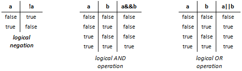
In order to be able to word more complex conditions logical operators are also needed besides relational operators. In language C++ the operation of logical AND (conjunction, &&), logical OR (disjunction, //) and negation (!) can be used when phrasing conditions.
The operation of logical operators can be described with a so called truth table:
The condition below is true if the value of variable x is between -1 and +1. Parentheses only confirm precedence.
-1 < x && x < 1
(-1 < x) && (x < 1)
There are cases when it is simpler to phrase the opposite condition instead of the condition itself, and apply a logical negation (NO) operator (!) on it. The condition of the previous example is identical with the condition below:
!(-1 >= x || x >= 1)
During logical negation all relations are changed to their opposite relation, while operator AND to operator OR (and vice versa).
In C++ programs numerical variable ok is frequently used in expressions
!ok instead of ok == 0
ok instead of ok != 0
Right side expressions are recommended to be used mainly with bool type variable ok.
I.3.6.3. Short circuit evaluation
The table of operations reveals that the evaluation of logical expressions is carried out from left to right. In case of certain operations, it is not necessary to process the whole expression in order to make the value of expression unambiguous.
Let’s take the example of operation logical AND (&&) during the usage of which the false (0) value of the left side operand makes the processing of the right side operand unnecessary. This evaluation method is called short circuit evaluation.
If there is a side effect expression on the right side of the logical operator during the evaluation, the
x || y++
result is not always what we expect. In the example above if the value of x is not zero y is not incremented. Short circuit evaluation takes place even if the operands of the logical operations are put in parentheses:
(x) || (y++)
I.3.6.4. Conditional operator
Conditional operator (?:) has three operands:
condition ? true_expression : false_expression
If the condition is true, the value of true_expression provides the value of the conditional expression, otherwise the false_expression after the colon (:). This way only one expression is evaluated out of the two expressions on the two sides of the colon. The type of the conditional expression is the same as that of the part with higher accuracy. The type of expression
(n > 0) ? 3.141534 : 54321L;
is always double independent of the value of n.
Let’s take a typical example for the application of the conditional operator. With the help of the expression below the values between 0 and 15 of variable n are transformed into hexadecimal numbers:
ch = n >= 0 && n <= 9 ? '0' + n : 'A' + n - 10;
It is to be noted that the precedence of conditional operation is relatively low, slightly precedes that of assignment, therefore parentheses should be used in more complex expressions:
c = 1 > 2 ? 4 : 7 * 2 < 3 ? 4 : 7 ; // 7 ↯
c = (1 > 2 ? 4 : (7 * 2)) < 3 ? 4 : 7 ; // 7 ↯
c = (1 > 2 ? 4 : 7) * (2 < 3 ? 4 : 7) ; //28
I.3.7. Bit operations
Computers had quite small memory in the past therefore solutions that made it possible to store and process more data within one byte, the smallest unit that can be addressed, were quite worthy. Using bit operations even 8 logical values can be stored within one byte. Nowadays this aspect is only considered rarely, easily understandable programs are in focus instead.
However, there is a field where bit operations are still used, and that is programming different hardware elements, microcontrollers. The C++ language contains six operators with the help of which different bitwise operations can be carried out on signed and unsigned integer data.
I.3.7.1. Bitwise logical operations
The first group of operations, the bitwise logical operations make it possible to test, delete or set bits:
|
Operator |
Operation |
|---|---|
|
|
Unary complement, bitwise negation |
|
|
bitwise AND |
|
|
bitwise OR |
|
|
bitwise exclusive OR |
The description of bitwise logical operations can be found in the table below, where 0 and 1 numerals denote deleted and set bit status, respectively.
|
a |
b |
a & b |
a | b |
a ^ b |
~a |
|---|---|---|---|---|---|
|
0 |
0 |
0 |
0 |
0 |
1 |
|
0 |
1 |
0 |
1 |
1 |
1 |
|
1 |
0 |
0 |
1 |
1 |
0 |
|
1 |
1 |
1 |
1 |
0 |
0 |
The low level control of the computer hardware elements requires setting, deletion and switching of certain bits. All these operations are called “masking” since an adequate bitmask should be prepared for every single operation, and then should also be linked logically with the value desired to be changed, and this way the desired bit operation takes place.
Before all conventional bit operations are described one after the other, bit numbering in integer data elements has to be discussed. Bit numbering in a byte starts from the smallest order bit from 0 and increases from right to left. In case of integers composed of more bytes the byte sequence applied by the processor of the computer should also be discussed.
In case “big-endian” byte sequence supported by Motorola 68000, SPARC, PowerPC etc. processors the most significant byte (MSB) is stored in the lowest memory address, while an order smaller byte in the next address and so on.
However, the members of the most widespread Intel x86 based processor family use “little-endian” byte sequence according to which the least significant byte (LSB) is stored in the lowest memory address.
In order to avoid long bit series unsigned short int type data elements are used in our examples. Let’s take a look at the structure and storing of these data according to both byte sequences. The stored data is 2012 that is 0x07DC in hexadecimal numbering.
big-endian byte sequence:
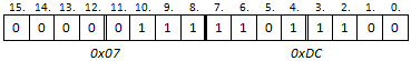
little-endian byte sequence:
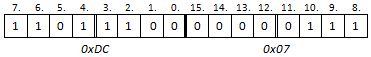
(Memory addresses increase from left to right in the example.) The figure shows clearly that when the hexadecimal constant values are entered the first big-endian form is used that corresponds to the mathematical interpretation of the hexadecimal number system. This is not an issue since storing in the memory is the task of the compiler. However, if the integer variables are processed bytewise, byte sequence should be known. Hereinafter our example programs are prepared in little-endian form but they can be adapted to the first storage method, as well based on the above mentioned facts.
In the example below bits 4 and 13 of the unsigned shortint type number 2525 are handled: unsigned short int x = 2525; // 0x09dd
|
Operation |
Mask |
C++ instruction |
Result |
|---|---|---|---|
|
Bit setting |
0010 0000 0001 0000 |
x = x | 0x2010; |
0x29dd |
|
Bit deletion |
1101 1111 1110 1111 |
x = x & 0xdfef; |
0x09cd |
|
Bit negation (switching) |
0010 0000 0001 0000 |
x = x ^ 0x2010; x = x ^ 0x2010; |
0x29cd (10701) 0x09dd (2525) |
|
Negation of all bits |
1111 1111 1111 1111 |
x = x ^ 0xFFFF; |
0xf622 |
|
Negation of all bits |
x = ~x; |
0xf622 |
Attention should be drawn to the strange behavior of exclusive or operator (^). If the exclusive or operation is carried out twice using the same mask the original value is returned, in this case 2525. This operation can be used for exchanging the values of two integer variables without the use of an auxiliary variable:
int m = 2, n = 7;
m = m ^ n;
n = m ^ n;
m = m ^ n;
A program error difficult to find is the result if the logical operators (!, &&, ||) used in conditions are interchanged with the bitwise operators (~, &, |).
I.3.7.2. Bit shift operations
Bit shift operators belong to another group of bit operations. Shift can be carried out either to the left (<<) or to the right (>>). During shifting the bits of the left side operand move to the left (right) as many times as the value of the right side operand shows.
In case of shifting to the left bit 0 is placed into the free bit positions, while the exiting bits are lost. However, shift to the right takes into consideration whether the number is signed or not. In case of unsigned types bit 0 enters from the left, while in case of signed numbers bit 1 comes in. This means that bit shift to the right keeps the sign.
short int x;
|
Value giving |
Binary value |
Operation |
Result decimal (hexadecimal) binary |
|---|---|---|---|
|
x = 2525; |
0000 1001 1101 1101 |
x = x << 2; |
10100 (0x2774) 0010 0111 0111 0100 |
|
x = 2525; |
0000 1001 1101 1101 |
x = x >> 3; |
315 (0x013b) 0000 0001 0011 1011 |
|
x = -2525; |
1111 0110 0010 0011 |
x = x >> 3; |
-316 (0xfec4) 1111 1110 1100 0100 |
If the results are examined it can be seen that due to shift to the left with 2 bits the value of variable x increased four (22) times, while shift to the right with three steps resulted in a value decrease of x to its eighth (23). It can be stated generally that if the bits of an integer number is shifted to the left by n steps, the result is the multiplication of that number with 2n. Shift to the right by m bits means integer division by 2m. It is to be noted that this is the fastest way to multiply/divide an integer number with/by 2n.
In the example below the 16-bit integer number is divided into two bytes:
  short int num;
  unsigned char lo, hi;

  // Reading the number
  cout<<"\nPlease enter an integer number [-32768,32767] : ";
  cin>>num;

  // Determination of the lower byte by masking
  lo=num & 0x00FFU;

  // Determination of the upper byte by bit shift
  hi=num >> 8;
In the last example the byte sequence of the 4 byte int type variable is reversed:
int n =0x12345678U;
n =     (n >> 24) |        // first byte is moved to the end,
    ((n << 8) & 0x00FF0000U) |    // 2nd byte into the 3rd
byte,
    ((n >> 8) & 0x0000FF00U) |    // 3rd byte into the 2nd byte,
    (n << 24);        // the last byte to the beginning.
cout <<hex << n <<endl;        // 78563412
I.3.7.3. Bit operations in compound assigment
In language C++ a compound assignmnet operation also belongs to all the five two-operand bit operations, and this way the value of variables can be modified more easily.
|
Operator |
Relation sign |
Usage |
Operation |
|---|---|---|---|
|
Assignmnet by shift left |
|
|
shift of bits of x to the left with y bits, |
|
Assignmnet by shift right |
|
|
shift of bits of x to the right with y bits, |
|
Assignmnet by bitwise OR |
|
|
new value of x: x | y, |
|
Assignmnet by bitwise AND |
|
|
new value of x: x & y, |
|
Assignmnet by bitwise exclusive OR |
|
|
new value of x: x ^ y, |
It is important to note that the type of the result of bit operations is an integer type, at least int or larger than int, depending on the left side operand type. In case of bit shift any number of steps can be entered but the compiler uses the remainder created with the bit size of the type for shifting. For example, the phenomenon listed below is experienced in case of 32 bit int type variables.
unsigned z;
z = 0xFFFFFFFF, z <<= 31; // z ⇒ 80000000
z = 0xFFFFFFFF, z <<= 32; // z ⇒ ffffffff
z = 0xFFFFFFFF, z <<= 33; // z ⇒ fffffffe
I.3.8. Comma operator
In one expression more, even independent expressions can be placed, using the lowest precedence comma operator. Expressions containing comma operator is evaluated from left to right, and the value and type of the expression is the same as that of the right side operand. Let’s take the example of expression
x = (y = 4 , y + 3);
Evaluation starts with the comma operator in the parentheses, first variable y obtains a value (4), then the expression in parentheses (4+3=7). Finally variable x obtains 7 as its value.
Comma operator is frequently used when setting different initial values for variables in one single statement (expression):
x = 2, y = 7, z = 1.2345 ;
Comma operator should be used also when the values of two variables should be changed within one statement (using a third variable):
c = a, a = b, b = c;
It is to be noted that commas that separate variable names in declarations and arguments in function calls are not comma operators.
I.3.9. Type conversions
It happens frequently during expression evaluation that a two-operand operation has to be carried out with different type operands. However, in order to be able to carry out the operation, the compiler has to transform the two operands to the same type, i.e. type conversion takes place.
In C++ some type conversions are carried out automatically without the intervention of the programmer, based on the rules laid in the definition of the language. These conversions are called implicit or automatic conversions.
In a C++ program the programmer may also request type conversion using type converter operators (cast) – explicit type conversion.
I.3.9.1. Implicit type conversions
It can be stated in general that during automatic conversions the operand with “narrower value range” is converted to the operand type with “wider value range” without data loss. In the example below during the evaluation of expression m+dint type m operand is converted to double type and that is the type of the expression as well:
int m=4, n;
double d=3.75;
n = m + d;
Implicit conversions do not always take place without data loss. During assigment and function call conversion among any types may happen. For instance in the example above when the sum is filled into variable n data loss occurs since the fraction part of the sum is lost, and 7 will be the value of the variable. (It is to be noted that no rounding was done during value giving.)
Automatically carried out conversions during evaluation of x op y form expressions are summarized briefly below.
char, wchar_t, short, bool, enum type data are automatically converted to int type. If the int type is not capable of storing the value, the aim type of conversion will be unsigned int. This type conversion rule is called “integer conversion” (integral promotion). The above mentioned conversions are value keeping ones, since they provide correct results regarding value and sign.
If there are different types in the expression after the first step, conversion according to type hierarchy starts. During type conversion the “smaller” type operand is converted to the “larger” type. The rules used during conversion are called “common arithmetical conversions”.
int < unsigned < long < unsignedlong < longlong < unsignedlonglong < float < double < long double
I.3.9.2. Explicit type conversions
The aim of type conversions commanded explicitly by the user is to carry out conversions that do not take place implicitly. Now only conversions that can be used with the basic types are dealt with, while operations const_cast, dynamic_cast and reinterpret_cast are detailed in Section I.6, “Pointers, references and dynamic memory management”.
The (static) type conversions below are all carried out during the compilation of the C++ program. A possible grouping of type conversions:
|
type conversion (C/C++) |
(type name) expression |
|
|
function-like form |
type name (expression) |
|
|
checked type conversions |
static_cast< type name >(expression) |
|
In case of writing any expression implicit and the maybe necessary explicit conversions have to be considered always. The program part below aims to determine the average of two long integer variables and store it as a double type variable:
long a =12, b=7;
double d = (a+b)/2;
cout << d << endl;    // 9
The result is false since due to integer conversions the right side of value giving has a long type result and this is placed into variable d. The result will only be right (9.5) if any operand of the division is converted to type double using any of the methods shown below:
d = (a+b)/2.0;
d = (double)(a+b)/2;
d = double(a+b)/2;
d = static_cast<double>(a+b)/2;
I.4. Control program structures
On the basis of what we have learnt so far, we can only make program codes in the main () function of which only contains expressions ending with semicolon (data input, value assignment, printing, etc.). In order to realize more complex algorithms, this program structure is insufficient. We have to get to know the control structures of the C++ language that make possible the execution of certain program code lines repeatedly or depending on certain conditions. (For a summary of all C++ statements, see Appendix Section A.5, “Statements in C++”.)
I.4.1. Empty statements and statement blocks
Control statements of C++ "control" the execution of other statements. If we would not like to control any activity, we should provide an empty statement. However, if several statements need control, then the so-called compound statements, i.e. statement blocks should be used.
Empty statements consist only of a semicolon (;). They should be used if no activity has to be performed logically, but there has to be a statement at the given point of the code according to syntax rules.
Curly brace brackets ( { and } ) enclose declarations and statements that make up a coherent unit together within a compound statement or block . Compound statements can be used at any place where only one statement is allowed in C++. Compound statements, the general representation of which is:
{
   local definitions, declarations
   statements
}
are used in the following three cases:
when more statements forming together a logical unit should be treated as one (in these cases, blocks only contain statements in general),
in the body of functions,
to localize the validity of definitions and declarations.
In the statement blocks statements and definitions/declarations can be typed in any order we want. (It should be noted that blocks do not end with a semicolon.)
In the following example, the quadratic equation with one unknown is solved if and only if the discriminant (the number appearing under the square root) of the equation is not negative. In order that the code would function correctly, the following if control structure is used:
#include <iostream>
#include <cmath>
using namespace std;

int main()
{
    double a, b, c;
    cout << "a = "; cin >> a;
    cout << "b = "; cin >> b;
    cout << "c = "; cin >> c;

    if (b*b-4*a*c>=0) {
        double x1, x2;
        x1 = (-b + sqrt(b*b-4*a*c))/(2*a);
        x2 = (-b - sqrt(b*b-4*a*c))/(2*a);
        cout << x1 << endl;
        cout << x2 << endl;
    }
}
I.4.2. Selective structures
Selective structures (if, switch) decide on the following steps to be executed by a program on the basis of certain conditions. These structures allow for one-way, two-way or multiple-way branches. Selections can be nested in one another, too. Conditions are expressed by comparison (relational) and logical operations.
I.4.2.1. if statements
In the case of an if statement, the execution of an activity (statement) depends on the value of an expression (condition). if statements have three forms
One-way branch
In the following form of if, the statement is only executed if the value of condition is not zero (i.e. true). (It should be noted that conditions should always be within brackets.)
if (condition)
statement
The functioning of the different control structures can be demonstrated by the following block diagram. The simple if statement is represented in Figure I.7, “Functioning of a simple if statement”.
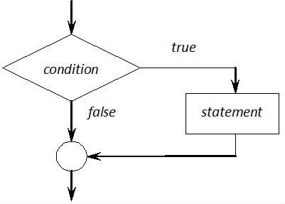
In the following example, the square root of the number read from the keyboard is only calculated if it is not negative:
#include <iostream>
#include <cmath>
using namespace std;

int main() {
  double x = 0;
  cout << "x = "; cin >> x;
  if (x >= 0) {
    cout<<sqrt(x)<<endl;
  }
}
Two-way branches
In the complete version of an if statement, an activity can be provided (statement2) when the value of the condition is zero (i.e. false) (Figure I.8, “Logical representation of if-else structures”). (If statement1 and statement2 are not compound statements, they should end with a semicolon.)
if (condition)
statement1
else
statement2
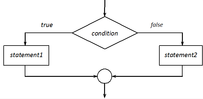
In the following example, the if statement decides whether the number read from the keyboard is even or odd:
#include <iostream>
using namespace std;

int main()
{
  int n;
  cout<<"Type an integer number: "; cin>>n;
  if (n % 2 == 0)
     cout<<"The number is even!"<<endl;
  else
     cout<<"The number is odd!"<<endl;
}
if statements can be nested in one another. However, in such cases, we have to be careful when using else branches. Compilers connect else branches to the closest preceding if statement.
The following example decides whether a given integer number is a positive and even number or whether it is a non-positive number. The correct solution can be realized in two different ways. One possibility is to attach an else branch containing an empty statement (;) to the internal if statement:
if (n > 0)
    if (n % 2 == 1)
        cout<<"Positive odd number."<< endl;
    else ;
else
    cout<<"Not a positive number."<<endl;
Another possibility is to enclose the internal if statement in braces, that is to place it in a statement block:
if (n > 0) {
    if (n % 2 == 1)
        cout<<"Positive odd number."<< endl;
} else
    cout<<"Not a positive number."<<endl;
This problem does not arise if statement blocks are used in the case of both if, which is by the way required by safe programming:
if (n > 0) {
    if (n % 2 == 1) {
        cout<<"Positive odd number."<< endl;
    }
}
else {
    cout<<"Not a positive number."<<endl;
}
In this case, both branches can be safely expanded by further statements.
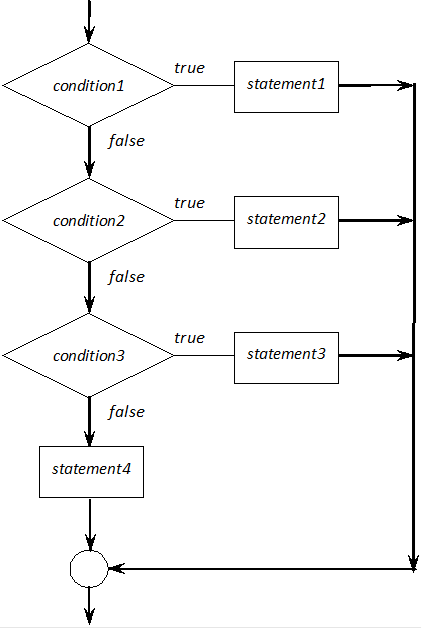
Multi-way branches
A frequent case of nested if statements is to use further if statements in else branches (Figure I.9, “Logical representation of multi-way branches”).
This structure realizes multi-way branches. If any condition is true, the corresponding statement is executed. If no condition is fulfilled, only the last else statement is executed.
if (condition1)
statement1
else if (condition2)
statement2
else if (condition3)
statement3
else
statement4
The following example decides whether number n is negative, 0 or positive:
if (n > 0)
    cout<<"Positive number"<<endl;
else if (n==0)
    cout<<"0"<<endl;
else
    cout<<"Negative number"<<endl;
A special case of else-if structures is when we check whether two elements are equal or not (==). The following example demonstrates a calculator counting the result of a simple addition and subtraction:
#include <iostream>
using namespace std;

int main()
{
    char op;
    double a, b, c;
    cout<<"expression : ";
    cin >>a>>op>>b;      // reading from keyboard: 4+10 <Enter>

    if (op == '+')
        c = a + b;
    else if (op == '-')
        c = a - b;
    else {
        cout << "Not a valid operator: " << op <<endl;
        return -1;
    }
    cout <<a<<op<<b<<'='<<c<<endl;
    return 0;
}
The following example counts the grades to be given to students on the basis of the achieved points in C++ programming:
#include <iostream>
using namespace std;

int main()
{
    int points
    char grade = 0;
    cout << "Points: ";  cin >> points;

    if (points >= 0 && points <= 100)
    {
        if (points < 40)
            grade = 'A';
        else if (points >= 40 && points < 55)
            grade = 'B';
        else if (points >= 55 && points < 70)
            grade = 'C';
        else if (points >= 70 && points < 85)
            grade = 'D';
        else if (points >= 86)
            grade = 'F';
        cout << "Grade: " << grade << endl;
    }
    else
        cout <<"Not a valid number!" << endl;
}
I.4.2.2. switch statements
In fact, switch statements are statement blocks that we can enter into depending on the value of a given integer expression. The parts of the code to be executed are determined by the so-called case labels (caseconstant expressions).
switch (expression)
{
caseconstant_expression1 :
statements1
caseconstant_expression2 :
statements2
caseconstant_expression3 :
statements3
default :
statements4
}
First, switch statements evaluate the expression, then transfer control to the case label in which the value of the constant_expression equals to the value of the evaluated expression. After that, all statements are executed from the entering point until the end of the block. If none of the case constants are equal to the value of the expression, control passes to the statement with label default. If no default label is provided, control passes to the statement following the brace closing the block of the switch statement.
This little bit weird functioning is demonstrated by an exceptional example code. The following switch statement is able to count the factorial of all integer numbers between 0 and 5. (In this case, the adjective exceptional means 'not to be followed'.)
int n = 4, f(1);
switch (n) {
    case 5: f *= 5;
    case 4: f *= 4;
    case 3: f *= 3;
    case 2: f *= 2;
    case 1: f *= 1;
    case 0: f *= 1;
}
In most cases switch statements are used, similarly to else-if structures, to realize multi-way branches. For that purpose, all statement blocks that correspond to a case have to end with a jump statement (break, goto or return). break statements transfer control to the statement immediately following the switch block, goto to the statement with the specified label within the function block and finally return exits the function.
Since our aim is to create well functioning and easily comprehensible source codes, the number of jump statements should be reduced to a minimum level. However, the usage of break is completely allowed in switch statements. In general, statements even at the end of the default label is followed by a break since the default case can be placed anywhere within switch statements.
On the basis of the above, the calculator program of the previous subsection can be rewritten by switch in the following way:
#include <iostream>
using namespace std;

int main()
{
    char op;
    double a, b, c;
    cout<<"expression :";
    cin >>a>>op>>b;

    switch (op) {
        case '+':
            c = a + b;
            break;
        case '-':
            c = a - b;
            break;
        default:
            cout << "Not a valid operator: " << op <<endl;
            return -1;
    }
    cout <<a<<op<<b<<'='<<c<<endl;
    return 0;
}
The next example demonstrates how to associate the same code part to more cases. In the source code, the case labels corresponding to cases 'y' and 'Y', as well as 'n' and 'N' were placed one after the other in the switch statement processing the response character.
#include <iostream>
using namespace std;

int main()
{
    cout<<"The response [Y/N]?";
    char response=cin.get();

    switch (response) {
        case 'y':  case 'Y':
            cout<<"The answer is YES."<<endl;
            break;
        case 'n':
        case 'N':
            cout<<"The answer is NO."<<endl;
            break;
        default:
            cout<<"Wrong response!"<<endl;
            break;
    }
}
I.4.3. Iteration structures (loops)
In programming, program structures ensuring automatic repetitions of statements are called iterations or loops. In C++, loop statements repeat a given statement in the function of the repetition condition until the condition is true.
while (condition) statement
for (initialisation opt ; condition opt ; increment_expression opt ) statement
dostatementwhile (condition)
In the case of for statement, opt means that the corresponding expressions are optional.
Loops can be classified on the basis of the place where control conditions are processed. Loops in which the control condition is evaluated before statements are executed are called pre-test loops. Any statement in the loop is executed if and only if the condition is true. Pre-test loops of C++ are while and for.
On the contrary, the statements of do loops are always executed at least once since control condition is evaluated after the execution of the statement – post-test loops.
In all three cases, correctly organized loops terminate if the control condition becomes false (0). However, there are times we create intentionally loops the control condition of which never becomes false. These loops are called infinite loops :
for (;;) statement;

while (true) statement;

do statement while (true);
Loops (even infinite loops) can be exited before the control condition becomes false. For that purpose, C++ offers statements like break, return or goto, which points to a place outside the body of the loop. Certain statements of the body of the loop can be bypass by using continue. The continue makes the program continue with executing the next iteration of the loop.
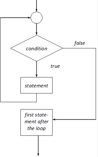
I.4.3.1. while loops
while loops repeat statements belonging to them (the body of the loop), while the value of the examined condition is true (not 0). Evaluation of the condition always precedes the execution of the statement. The process of the functioning of while loops can be traced in Figure I.10, “Logical representation of while loops”.
while (condition)
statement
The next example code determines the sum of the first n natural numbers:
#include <iostream>
using namespace std;

int main()
{
    int n = 2012;
    cout<<"The sum of the first "<<n<<" natural number ";
    unsigned long sum = 0;
    while (n>0) {
        sum += n;
        n--;
    }
    cout<<"is: "<<sum<<endl;
}
Of course, the while loop of the previous example can be simplified but this step decreases its readability:
|
|
|
|
C++ makes it possible to place variable declarations anywhere in a program code. The only condition is that all variables have to be declared (defined) before they are used. In certain cases, variables can be defined in loop statement header in case they are immediately initialized, e.g. by random numbers.
The while loop of the following example code does not terminate until it reaches the first number, divisible by 10. In the code, statement
srand((unsigned)time(NULL));
initializes the random number generator with the actual time, therefore every execution result in a new number sequence. Random numbers are provided by function rand () in the value range between 0 and RAND_MAX (32767).
#include <iostream>
#include <cstdlib>
#include <ctime>
using namespace std;

int main()
{
    srand((unsigned)time(NULL));
    while (int n = rand()%10)
        cout<< n<< endl;
}
It should be noted that variable n defined in that way can be accessed within the while loop, thus it is local only with respect to the while loop.
I.4.3.2. for loops
In general, for statements are used if the statements within its body should be executed in a given number of times (Figure I.11, “Logical representation of for loops”). In the general form of for statements, the role of each expression is also mentioned:
for (initialization; condition; increment)
statement
In reality, for statements are the specialized versions of while statements, so the above for loop can perfectly be transformed into a while loop:
initialization;
while (condition) {
statement;
increment;
}
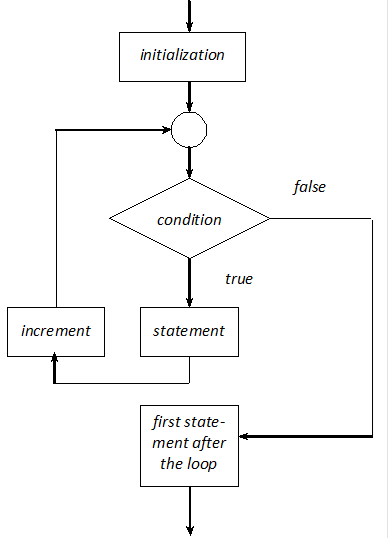
The following program represents a for loop and does the same as the above one: determines the sum of natural numbers. It is obvious at first sight that this solution of the problem is much more readable and simpler:
#include <iostream>
using namespace std;

int main()
{
    unsigned long sum;
    int i, n = 2012;
    cout<<"The sum of the first "<<n<<" natural number ";
    for (i=1, sum=0 ; i<=n ; i++)
        sum += i;
    cout<<"is: "<<sum<<endl;
}
There is only one expression-statement in the body of the loop in the example, so the for loop can be condensed in the following way:
for (i=1, sum=0 ; i<=n ; sum += i, i++) ;
or
for (i=1, sum=0 ; i<=n ; sum += i++) ;
Loops can be nested in one another, since their body can contain other loop statements. The following example uses nested loops to print a pyramid of a given size. In all three loops, loop variable is made local:
#include <iostream>
using namespace std;

int main ()
{
    const int maxn = 12;
    for (int i=0; i<maxn; i++) {
        for (int j=0; j<maxn-i; j++) {
            cout <<" ";
        }
        for (int j=0; j<i; j++) {
            cout <<"* ";
        }
        cout << endl;
    }
}
|
            *
           * *
          * * *
         * * * *
        * * * * *
       * * * * * *
      * * * * * * *
     * * * * * * * *
    * * * * * * * * *
   * * * * * * * * * *
  * * * * * * * * * * *
|
I.4.3.3. do-while loops
In do-while loops, evaluation of the condition takes place after the first execution of the body of the loop (Figure I.12, “Logical representation of do-while loops”), so the loop body is always executed at least once.
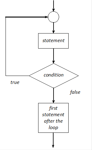
do
statement
while (condition);
As a first step, let's create the version of the program computing the sum of natural numbers with a do-while loop.
#include <iostream>
using namespace std;

int main()
{
    int n = 2012;
    cout<<"The sum of the first "<<n<<" natural number ";
    unsigned long sum = 0;
    do {
        sum += n;
        n--;
    } while (n>0);
    cout<<"is: "<<sum<<endl;
}
With the help of the following loop, let's read an integer number between 2 and 100 from the input and verify it:
int m =0;
do {
    cout<<"Enter an integer number betwwen 2 and 100: ";
    cin >> m;
} while (m < 2 || m > 100);
The last example calculates the power of a number with an integer exponent:
#include <iostream>
#include <cstdlib>
using namespace std;

int main()
{
    double base;
    int exponent;
    cout << "base:  "; cin >> base;
    cout << "exponent:  "; cin >> exponent;
    double power = 1;
    if (exponent != 0)
    {
        int i = 1;
        do
        {
            power *= base;
            i++;
        } while (i <= abs(exponent));
        power = exponent < 0 ? 1.0 / power : power;
    }
    cout <<"The power is :  " << power << endl;
}
A frequent programming error is to terminate loop headers with a semicolon. Let's see some attempts to print odd integer numbers between 1 and 10.
|
|
|
|
In the case of while, the empty statement is repeated endlessly in the loop. The for loop repeats the empty statement and then prints the value of the loop variable after the loop is exited, i.e. 11. In the case of the do-while loop, the compiler gives an error message if do is followed by a semicolon, so the example code is a perfect solution.
I.4.3.4. break statements in loops
There are cases when the regular functioning of a loop has to be directly intervened into. For example, if a loop has to be exited if a given condition is fulfilled. A simple solution for that is the break statement, which interrupts the execution of the nearest while, for and do-while statements and control passes to the first statement following the interrupted loop.
The following while loop is interrupted if the lowest common multiple of two integer numbers is found:
#include <iostream>
#include <cstdlib>
using namespace std;

int main()
{
    int a, b, lcm;
    cout << "a = "; cin >> a;
    cout << "b = "; cin >> b;
    lcm = min(a,b);
    while (lcm<=a*b) {
        if (lcm % a == 0 && lcm % b == 0)
            break;
        lcm++;
    }
    cout << "The lowest common multiple is: " << lcm << endl;
}
The usage of break can be avoided if the condition of the if statement corresponding to it can be integrated into the condition of the loop, that will become more complicated by that step:
    while (lcm<=a*b && !(lcm % a == 0 && lcm % b == 0)) {
        lcm++;
    }
If break statement is used in nested loops in an inner loop, it is only that inner loop that is exited. The following example prints prime numbers between 2 and maxn. The reason for exiting the loop is provided by a logical flag, by the variable (prime), to the outer loop:
#include <iostream>
using namespace std;

int main () {
    const int maxn =2012;
    int divisor;
    bool prime;
    for(int num=2; num<=maxn; num++) {
        prime = true;
        for(divisor = 2; divisor <= (num/divisor); divisor++) {
            if (num % divisor == 0) {
                prime = false;
                break; // has a divisor, not a prime
            }
        }
        if (prime)
cout << num << " is a prime number" << endl;
    }
}
If the task is to find the first Pythagorean triple in a given interval, two for loops have to be exited if a match is found. Then the simplest solution is to use the flag (found):
#include <iostream>
#include<cmath>
using namespace std;

int main () {
    int left, right;
    cout <<"left  = "; cin >> left;
    cout <<"right = "; cin >> right;
    bool found = false;
    for(int a = left, c, c2; a<=right && !found; a++) {
        for(int b = left; b<=right && !found; b++) {
            c2 = a*a + b*b;
            c = static_cast<int>(sqrt(float(c2)));
            if (c*c == c2) {
                found = true;
                cout << a << ", " << b  << ", " << c << endl;
            } // if
        } // for
    } // for
} // main()
I.4.3.5. continue statements
continue statements start the next iteration of while, for and do-while loops. In the body of these loops, the statements placed after continue are not executed.
In the case of while and do-while loops, the next iteration begins with evaluating again the condition. However, in for loops, the processing of the condition is preceded by the increment.
In the following example, with the help of continue, it was realized that only the numbers divisible by 7 or 12 are printed out in the loop incrementing from 1 to maxn by one:
#include <iostream>
using namespace std;

int main(){
    const int maxn = 123;
    for (int i = 1; i <= maxn; i++) {
        if ((i % 7 != 0) && (i % 12 != 0))
            continue;
        cout<<i<<endl;
    }
}
It is a bad practice in programming to use often break and continue statements. It has to be always rethought if given program structures can be solved without jump statements. In the preceding example, this can easily be done by inverting the condition of the if statement:
    for (int i = 1; i <= maxn; i++) {
        if ((i % 7 == 0) || (i % 12 == 0))
            cout<<i<<endl;
    }
I.4.4. goto statements
To close the present chapter, let's see one jump statement of C++ not presented yet. We should already be careful when using break and continue statements, but this is even truer for goto statements.
goto statements that can be used to jump within functions have a bad reputation because they make program codes less understandable and more unstructured. Not to mention the tragic consequences of jumping into a loop. So, it should be stated that goto statements are to be avoided if a structured and a clearly understandable code is to be written. In most software developer companies, it is even forbidden.
In order to use goto statements, the statement to which we want to jump has to be labeled. A label is an identifier which is separated by a colon from the following statement:
label: statement
The goto statement with which control can be transferred to the line marked with the label above:
goto label;
In some and only justified cases, e.g. jumping out from a very complicated program structure, goto provides a simple alternative.
I.5. Exception handling
An anomalous state or event that hinders the normal flow of the execution of a program is called an exception.
In C language, errors were handled locally at every eventual anomalous point of a program. In general, this meant printing out an error message ( cerr ) and then interrupting the execution of that program ( exit ()). For example, when all coefficients of a quadratic equation have been read from the keyboard and the quadratic coefficient is 0, then the quadratic formula cannot be applied to solve the equation:
#include <iostream>
#include <cstdlib>
using namespace std;

int main()
{
    double a, b, c;
    cout<<" coefficients (separated from each"
           "other by a space) :";
    cin >> a >> b >> c;
    if (0 == a) {
        cerr << "The equation is not quadratic!" << endl;
        exit(-1);
    }
    cout <<a<<"x^2+"<<b<<"x+"<<c<<"=0"<< endl;
}
C++ makes it possible to assign types to exceptions (errors) and to carry out all exception handling tasks at the same place. Exception handling takes place on the basis of the termination model, which means that the execution of the code part (function) that provoked an exception is interrupted when that exception arises.
Standard C++ language contains relatively few integrated exceptions; however, different class libraries prefer exceptions to signal erroneous states. Exceptions can be triggered manually by "throwing" a value of a given type. Exceptions are transferred (thrown) to the nearest exception handlers that either catch or transfer them.
This above mentioned process functions only if the code part susceptible to trigger an error is enclosed in a statement block that attempts (try) to execute that.
So, the three elements that are needed for the type-oriented exception handling of C are the following:
selecting the code part under exception inspection (try-block),
transferring exceptions (throw),
catching and handling exceptions (catch).
I.5.1. The try – catch program structure
In general, a try-catch program structure contains only one try block and any number of catch blocks:
try
{
// statements under exception inspection
statements
}
catch (exception1 declaration) {
// the handler of exception1
statements1
}
catch (exception2 declaration) {
// the handler of exception2
statements2
}
catch (...) {
// the handler of any other exception
statements3
}
// statements that are executed after successful handling
statements4
In case any statement of a try block causes an exception, the execution of statements is interrupted and control is passed to the catch block (that follows that try block) of the given type (if there is one). If there is no handler with the given type, then the exception is transferred to a handler belonging to an external try block. Exceptions without any type match are finally transferred to the execution environment (as unhandled exceptions). This situation is signalled by the following message: "This application has requested the Runtime to terminate it in an unusual way. Please contact the application's support team for more information.”
The exception declarations that follow the keyword catch can be provided in many ways. These declarations may contain a type , a variable declaration (type identifier) or three dots . The thrown exception can only be accessed by using the second form. The three dots means that that block catches any exception. Since exceptions are identified in the order catch blocks are provided, the three dotted version should be the last in the catch-block list.
As an example, let's transform the error inspection of the introduction part into an exception handling.
#include <iostream>
#include <cstdlib>
using namespace std;

int main()
{
    try {
        double a, b, c;
        cout << " coefficients (separated from each"
                "other by a space) :";
        cin >> a >> b >> c;
        if (0 == a) throw false;
        cout <<a<<"x^2+"<<b<<"x+"<<c<<"=0"<< endl;
    }
    catch (bool) {
        cerr << "The equation is not quadratic!" << endl;
        exit(-1);
    }
    catch (...) {
        cerr << "An error occurred..." << endl;
        exit(-1);
    }
}
I.5.2. Provoking exceptions - the throw statement
Exceptions have to be handled locally within the given part of a code with the keywords try, throw and catch. Exception handling only takes place in case the code in the catch block (and the code called from there) is executed. From the selected code portion, a throw statement
throwexpression;
passes control to the handler that corresponds to the type of the expression, which should be provided after the keyword catch.
When an exception is transferred by a throw statement, then the value of the expression given in the statement is copied into the parameter figuring in the header of the catch block, so this value can be processed in that specific handler. For that purpose, the type also has to have an identifier in that catch statement.
If a catch block contains a throw statement, the caught exception can be transferred as another exception, either transformed to another or not. If the exception is not intended to be transformed, the empty throw statement has to be used: throw;
Exception handling can be made more complete by defining exception classes. The header file named exception contains the description of the exception class, which is the base class of different logical and run-time exceptions. The function named what () of these classes returns the string identifying that exception. The following table summarises the exceptions thrown by the classes defined in the C++ standard library. All exceptions have the exception class as their base class.
|
Exception classes |
Header file | ||
|---|---|---|---|
|
exception |
<exception> | ||
|
bad_alloc |
<new> | ||
|
bad_cast |
<typeinfo> | ||
|
bad_typeid |
<typeinfo> | ||
|
logic_failure |
<stdexcept> | ||
|
domain_error |
<stdexcept> | ||
|
invalid_argument |
<stdexcept> | ||
|
length_error |
<stdexcept> | ||
|
out_of_range |
<stdexcept> | ||
|
runtime_error |
<stdexcept> | ||
|
range_error |
<stdexcept> | ||
|
overflow_error |
<stdexcept> | ||
|
underflow_error |
<stdexcept> | ||
|
ios_base::failure |
<ios> | ||
|
bad_exception |
<exception> | ||
Exception classes make it possible to pass "smart" objects as exceptions instead of simple values. The knowledge necessary for that process is only treated in Chapter III, Object-oriented programming in C++ of the present book.
A comfortable way of exception handling is when a string is passed as exception. In that way, the users of a computer program will always receive meaningful messages during their work. (String constants will be declared as of type const char *, which will be treated in the next chapter.)
#include <iostream>
#include <cstdlib>
#include <ctime>
using namespace std;

int main() {
    int number;
    srand(unsigned(time(NULL)));
    try {
        while (true) {
            number = rand();
            if (number>1000)
                throw "The number is too big";
            else if (number<10)
                throw "The number is too small";
            cout << 10*number << endl;
        } // while

    } // try
    catch (const char * s) {
        cerr << s << endl;
    } // catch
} // main()
I.5.3. Filtering exceptions
Functions in C++ have an important role in exception handling. An exception arising in a function is generally processed within that function since related data are only available from there. However, there are some exceptions that indicate an unsuccessful working of the function back to the element that called the latter. Of course, these exceptions are transferred outside the function.
In the header of a function definition, the keyword throw can be used in a specific way, so the type of the exception to be thrown to the handler can also be defined. By default, all exceptions are transferred.
// all exceptions are transferred.
int funct1();
// only exceptions of type char and bool are transferred
int funct2() throw(char, bool);
// only exceptions of type bool are transferred
int funct3() throw(bool);
// no exceptions are transferred
int funct4() throw();
When a program throws an exception that does not have a handler in that program, the execution environment activates the function named terminate (), which makes the program abort ( abort ()). If a function body throws an exception that is not listed in the exceptions of the given function to be thrown, then the unexpected () system call terminates the program. Programmers can intervene in both terminating process by defining their own handlers that can be registered with the help of the functions set_terminate () or set_unexpected () declared in the header file named except.
I.5.4. Nested exceptions
A try-catch exception handling structure can be placed within another try-block, either directly or indirectly (i.e. in the function called from that try-block).
As an example, a string exception is thrown from an inner try-block. This is then processed in the inner structure and then transferred by using the empty throw; statement. The outer structure treats that exception finally.
#include <iostream>
using namespace std;

int main()
{
    try {
        try {
            throw "exception";
        }
        catch (bool) {
            cerr << "bool error" << endl;
        }
        catch(const char * s) {
            cout << "inner " << s << endl;
            throw;
        }
    }
    catch(const char * s) {
        cout << "outer " << s << endl;
    }
    catch(...) {
        cout << "unknown exception" << endl;
    }
}
As the final example of the present section, let's have a look at the following calculator program. Our own exceptions are stored in enumerations. The program can be exited by using the operator x.
#include <iostream>
using namespace std;
enum zerodiv {DividingWithZero};
enum wrongoperation {WrongOperation};
int main()
{
    double a, b, e=0;
    char op;
    while (true)  // exiting if op is x or X
    {
        cout << ':';
        cin >>a>>op>>b;
        try {
            switch (op) {
                case '+':    e = a + b;
                        break;
                case '-':    e = a - b;
                        break;
                case '*':    e = a * b;
                        break;
                case '/':    if (b==0)
                        throw DividingWithZero;
                        else
                            e = a / b;
                        break;
                case 'x': case 'X' :
                        throw true;
                default: throw WrongOperation;
            }
            cout << e <<endl;
        } // try
        catch (zerodiv) {
            cout <<" Dividing with zero" <<endl;
        }
        catch (wrongoperation) {
            cout <<" Wrong operation" <<endl;
        }
        catch (bool) {
            cout<<"Off"<<endl;
            break;   // while
        }
        catch(...) {
            cout<<" Something is bad "<< endl;
        }
    } // while
}
I.6. Pointers, references and dynamic memory management
The most important resource of every program is computer memory since all directly accessible (on-line) data is stored there along with executed program code. In our previous examples, it is compiler that was entrusted with memory management.
|
Based on the storage class, compiler places global (extern) data grouped together on a memory place which is always accessible while the program is running. Local (auto) data are stored in a stack memory block when the corresponding functions are entered into and they are deleted when these functions are exited (Figure I.13, “C++ program memory usage”). However, there is a space named heap, where programmers can place variables and delete those that are not needed anymore. These dynamically managed variables are different from those used so far since they have no name. They can be referenced by variables storing their address (pointers). C++ has a couple of operators that make dynamic memory management possible: *, &, new, delete. |
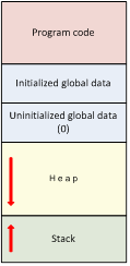 Figure I.13. C++ program memory usage
|
Besides the above mentioned areas, there are many domains where pointers are used in C/C++ programs: function parameter passing, linked data structure management, etc. C++ attempts to counterbalance the exclusive usage of pointers with the help of a safer type, namely with the help of references.
I.6.1. Pointers
When defining a variable, compilers reserve the quantity of memory space that corresponds to the type of the given variable and associate to the latter the name used in its definition. In most cases, we assign values to variables and read their content by using their names. There are cases where this approach is insufficient and the address of a variable in the memory should be used directly (for example when calling the Standard Library function scanf ()).
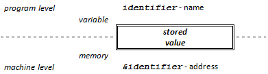
With the help of pointers, the address of variables (data stored in memory) and functions can be stored and managed. A pointer does not only store address but also have information how to interpret how many bytes from that given address. And this is the type of the referenced data, which is provided in the definition of pointers (variables).
I.6.1.1. Single indirection pointers
First, let's start with the most frequently used and the simplest form of pointers, that is with single indirection pointers the general definition of which is:
type *identifier;
The asterisk indicates that now a pointer is defined, and the type before the asterisk indicates the referenced data type. The default automatic initial value of pointers is determined by the usual rules: it is 0, if it is created outside functions and undefined when created within a function. It is a safe solution to initialize always pointers after they are created with NULL value, which can be found in most header files:
type *identifier = NULL;
If more pointers are created within a single statement, all identifier names should be preceded by an asterisk:
type *identifier1, *identifier2;
Many operations can be carried out for pointers; however, there are three operators that can exclusively be used with pointers:
|
*ptr |
Accessing the object ptr points to. |
|
ptr->member |
The access of the given member of the structure ptr points to (Section I.8, “User-defined data types”). |
|
&leftvalue |
Getting the address of leftvalue. |
The two levels presented in the introduction become more understandable if they are demonstrated by an example. Let's create an integer type variable.
int x = 2;
When the variable is defined, an (int type) space is created in memory (e.g. with the address of 2004) into which the initial value is copied:
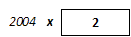
The definition of
int *p;
creates a variable (e.g. at the address of 2008), the type of which is int*. C++ generally considers p as an int* type variable or p can also be considered as an int type pointer. This pointer can be used for storing address of int type variables, that can be accessed by the "address of" & operation, e.g.
p = &x;
After that operation, the x name and *p value reference the same memory space. (the expression *p designate the storage place „p points to”.)
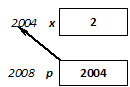
As a consequence, after the processing of
*p = x +10;
the value of x becomes 12.
An alternative pointer type can also be created by using the keyword typedef:
int x = 2;
typedef int *tpi;
tpi p = &x;
A single variable can be referenced by many pointers and its value can be modified by any of them:
int x = 2;
int * p, *pp;
p    = &x;
pp   = p;
*pp += 10; // the value of x is 12 again
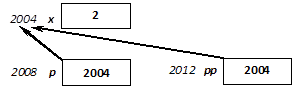
If a pointer is initialized with an address of a variable of a different type, a compiler error message is sent.
long y = 0;
char *p = &y;     // error! ↯
If it is not an error and the long type data is to be accessed by bytes, compilers can be asked to do value assignment by type cast:
long y = 0;
char *p = (char *)&y;
or
char *p = reinterpret_cast<char *>(&y);
It is a frequent error to use a pointer without initialization. In general, this results in the interruption of the execution of the program:
int *p;
*p = 1002;  // ↯ ↯ ↯
I.6.1.2. Pointer arithmetic
Besides the already presented operators (* and &), other ones can also be used. These operations together are covered by pointer arithmetic. Every other operation results in an undefined result, so they are to be avoided.
The allowed pointer arithmetic operations are summarised in a table where q and p are pointers (not of void* type), n is an integer number (int or long):
|
Operation |
Expression |
Result |
|---|---|---|
|
two pointers of the same type can be subtracted from each other |
q - p |
integer number |
|
an integer number can be added to a pointer |
p + n, p++,++p, p += n, |
pointer |
|
an integer number can be subtracted from a pointer |
p – n, p--, --p, p -= n |
pointer |
|
two pointers can be compared |
p == q, p > q, etc. |
bool (false or true) |
When an integer number is added to or subtracted from a pointer, compilers automatically scale the integer number according to the type of the pointer, therefore the stored address is not modified by n bytes but by
n * sizeof(pointer_type)
bytes, so the pointer "steps" by the size of n elements in memory.
Accordingly, increment and decrement operators can also be used for pointers and not only for arithmetic types, but in the former case it means going to the neighbouring element and not an increment or decrement by one byte.
Incrementing a pointer to the neighbouring element can be carried out in many ways:
int *p, *q;
p  = p + 1;
p += 1;
p++;
++p;
Decrementing to the preceding element can also be done in many ways:
p  = p - 1;
p -= 1;
p--;
--p;
Scaling also works when the difference of two pointers is counted, so we get the number of elements between the two pointers as a result:
int h = p - q;
I.6.1.3. void * type general pointers
C++ also allows for using general pointers without a type (void types),
int x;
void * ptr = &x;
which only store addresses, so they are not associated to any variable.
C++ ensures two implicit conversions for pointers. A pointer with any type can be transformed into a general (void) type pointer, and all pointers can be initialized by zero (0). For a conversion in the other direction, explicit type cast should be used.
That is why, if a value is to be given to variable referenced by ptr, the address should be associated with a type by a manual type cast. Type cast can be done in many ways:
int x;
void *ptr = &x;

*(int *)ptr = 1002;

typedef int * iptr;
*iptr(ptr) = 1002;

*static_cast<int *>(ptr) = 1002;

*reinterpret_cast<int *>(ptr) = 1002;
After any of these indirect value assignments, the value of x becomes 1002.
It should be noted that most of the functions in the Standard Library that return pointer are of void* type.
I.6.1.4. Multiple indirection pointers
Pointers can also be used in the case of multiple indirection relations. In these cases, the definition of pointers contains more asterisks (*):
type * *pointer;
The asterisk standing immediately before the pointer indicates that a pointer is defined, and what can be found before this asterisk is the type of the pointer (type *). Similarly to that, any number of asterisks can be interpreted to but in order to ease our readers, we note that the elements of C++ Standard Library use double indirection pointers at most.
Let's have a look at some definitions and let's find out what the created variable is.
|
int x; |
x is an int type variable, |
|
int *p; |
p is an int type pointer (that can point to an int variable), |
|
int * *q; |
q is an int* type pointer (that may point to an int* variable, that is to a pointer pointing to an integer). |
The above detailed definitions can be rewritten in a more understandable way by alternative (typedef) type names:
// iptr - pointer type pointing to an integer
typedef int *iptr;
iptr p, *q;
or
// iptr - pointer type pointing to an integer
typedef int *iptr;

// type of a pointer pointing to an iptr type variable
typedef iptr *ipptr;

iptr p;
ipptr q;
|
When these definitions are provided, and when the statements x = 2; p = &x; q = &p; x = x + *p + **q; are executed, the value of x will be 6. |
|
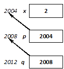
It should be noted that when interpreting more complex pointer relations, graphical representations provide a useful help.
I.6.1.5. Constant pointers
C++ compilers strictly verify the usage of const type constants, for example a constant can be referenced by an appropriate pointer:
const double pi = 3.141592565;
// pointer pointing to a double type data
double *ppi = π          // error! ↯
The assignment can be carried out by a pointer pointing to the constant:
// pointer pointing to a double constant
const double *pdc;
const double dc = 10.2;
double   d = 2012;
pdc  = &dc;                   // pdc pointer points to dc
cout <<*pdc<<endl;         // 10.2
pdc  = &d;                    // pdc pointer is set to d
cout <<*pdc<<endl;         // 2012
By using the pdc pointer, we cannot modify the value of the d variable:
*pdc = 7.29; // error! ↯
It is a pointer with a constant value, so the value of the pointer cannot be changed:
int month;
// constant pointer pointing to an int type data
int *const actmonth = &month; //
The value of the actmonth pointer cannot be changed only that of *actmonth.
*actmonth = 9;
cout<< month << endl;        // 9
actmonth = &month;           // error! ↯
Pointer with a constant value pointing to a constant:
const int month = 10;
const int amonth = 8;
// constant pointer pointing to an int type constant
const int *const actmonth = &month;
cout << *actmonth << endl;    // 10
Neither the pointer, nor the referenced data can be changed.
actmonth = &amonth;         // error! ↯
*actmonth = 12;             // error! ↯
I.6.2. References
Reference types make it possible to reference already existing variables while defining an alternative name. The general form of their definition:
type &identifier = variable;
& indicates that a reference is defined, while the type before the & designates the type of the referenced data that have to be the same as that of the variable set as its initial value. When defining many references with the same type, the sign & should be typed before all references:
type &identifier1 = variable1, &identifier2 = variable2 ;
When a reference is defined, initialisation has to be done with a left value. Let's make a reference to the int type x variable as an example.
int x = 2;
int &r = x;
Contrary to pointers, no variable is created to store references in general. Compilers just give a new name as a second name to the variable x (r).
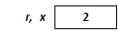
As a consequence, the value of x becomes 12 when the following statement is evaluated:
r = x + 10;
While the value of a pointer, and the referenced storage place as a consequence, can be modified at any time, the reference r is bound to a variable.
int x = 2, y = 4;
int &r = x;
r = y;            // normal value assignment
cout << x << endl;     // 4
If a reference is initialized by a constant value or a variable of a different type, a compiler error message is sent. It does not even help if type cast is used in the latter case. These cases are treated by compilers if a so-called constant (read-only) reference is created. In that case, the compiler creates first the storage place of the same type as that of the reference, then it initializes it with the right value standing after the equal sign.
const char &lf = '\n'; |
unsigned int b = 2004; const int &r = b; b = 2012; cout << r << endl; // 2004 |
Synonymous reference types can also be created by the keyword typedef:
typedef int &rint;
int x = 2;
rint r = x;
References can be created to pointers just like for other variable types:
int n = 10;
int *p = &n;        // p points to the variable n
int* &rp = p;        // rp is a reference to the pointer p
*rp = 4;
cout << n << endl;    // 4
The same can be done with typedef:
typedef int *tpi;     // type of a pointer pointing to an integer
typedef tpi &rtpi;    // reference to a pointer pointing to an integer
int n = 10;
tpi p = &n;
rtpi rp = p;
It should be noted that a reference or a pointer cannot be defined for a reference.
int n = 10;
int &r = n;
int& *pr = &r;       // error! ↯
int& &rr =r;        // error! ↯
int *p = &r;
// pointer p points to n via the reference r
Reference cannot be created for bitfields (Section I.8, “User-defined data types”), and we cannot even define an array consisting of reference elements (Section I.7, “Arrays and strings”).
We will experience the real significance of reference types when creating functions.
I.6.3. Dynamic memory management
In general, pointers are not used to point to other variables but it can also happen (e.g. when parameters are passed). Pointers are the key to one of the most important facilities of C++, namely to dynamic memory management. With pointers, it is programmer who allocates memory space necessary for the execution of a program and it is him who frees it if they are not needed anymore.
The dynamic management of free memory (heap) is a vital part of all programs. C ensures Standard Library functions for the needed memory allocation ( malloc (),...) and deallocation ( free ()) operations. In C++, the operators new and delete replace the above mentioned library functions (although the latter are also available).
Dynamic memory management consists of the following three steps:
allocating a free memory block while verifying the success of the allocation,
accessing the memory space with a pointer,
freeing (deallocating) the previously allocated memory space.
I.6.3.1. Allocating and accessing heap memory
The first step of dynamic memory management is allocating a memory space of the necessary size from the heap memory. For that purpose, the operator new can be used. The operator new allocates a memory space in the heap of the size corresponding to the type provided in its operand and returns a pointer pointing to the beginning of that memory space. If needed, an initial value can also be provided in the parentheses following the type.
pointer = newtype;
pointer = newtype(initial value);
new cannot only allocate memory space for one element but also for many elements standing one after the other. The data structure created in this way is called a dynamic array (Section I.7, “Arrays and strings”).
pointer = newtype[number_of_elements];
Let's see some examples for the operation new.
int main() {
    int *p1;
    double *p2;
    p1 = new int(2);
    p2 = new double;
}
The above mentioned definitions result in the creation of the pointer variables p1 and p2 in the stack. After value assignment, two dynamic variables are born in the stack memory. Their address appear in the corresponding pointers (Figure I.14, “Dynamic memory allocation”).
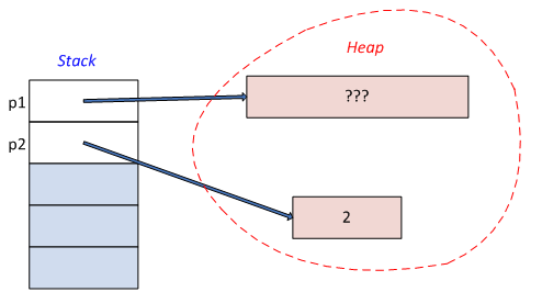
When memory space is allocated, especially for a big sized dynamic array, it may happen that there is no enough contiguous free memory at our disposal. C++ run-time system signals this issue by throwing a bad_alloc exception (exception header file). Program codes can be therefore made safe by using exception handling methods.
#include <iostream>
#include <exception>
using namespace std;

int main() {
   long * pdata;
   // Memory allocation
   try {
     pdata = new long;
   }
   catch (bad_alloc) {
      // Unsuccessful allocation
      cerr << "\nThere is no enough memory!" << endl;
      return -1;  // Program is exited
   }
   // ...
   // Deallocating (freeing) allocated memory space
   delete pdata;
   return 0;
}
If we do not benefit from exception handling opportunities, the nothrow constant should be used as an argument for the new operator (new header file). As a result, the new operator returns a 0 value instead of throwing an exception when memory allocation is unsuccessful.
#include <iostream>
#include <new>
using namespace std;

int main() {
   long * pdata;
   // Memory allocation
   pdata = new (nothrow)long;
   if (0 == pdata) {
      // Unsuccessful allocation
      cerr << "\nThere is no enough memory!" << endl;
      return -1;  // Program is exited
   }
   // ...
   // Deallocating (freeing) allocated memory space
   delete pdata;
   return 0;
}
Finally, we should not forget about another possibility of the new operator. new can also be followed directly by a pointer in parenthesis, which makes the operator return the value of the pointer (thus it does not allocate memory):
int *p=new int(10);
int *q=new(p) int(2);
cout <<*p << endl;   // 2
In the examples above, the pointer q reference the memory space p points to. Pointers can be of a different type:
long a = 0x20042012;
short *p = new(&a) short;
cout << hex <<*p << endl;  // 2012
I.6.3.2. Deallocating allocated memory
Memory blocks allocated by the operator new can be deallocated by the operator delete:
delete pointer;
delete[] pointer;
The first form of the operation is used to deallocate one single dynamic variable, whereas the second one is used in the case of dynamic arrays.
delete operation also works correctly with pointers of 0 value. In every other case where the value was not assigned by new, the result of delete is unpredictable.
The introductory example of the previous section can be made complete if memory space is deallocated:
int main() {
    int *p1;
    double *p2;
    p1 = new int(2);
    p2 = new double;
    delete p1;
    delete p2;
    p1 = 0;
    p2 = 0;
}
I.7. Arrays and strings
The variables in our previous examples were only able to store one (scalar) value at a time. Programming work often requires to store data sets comprising many similar or different elements in memory and to do operations on them. In C++, these tasks can efficiently be realised with the help of arrays and user-defined types (struct, class, union, see Section I.8, “User-defined data types”), that is derived types.
I.7.1. C++ array types
An array is a set of data of the same type (elements) that are placed in memory in a linear sequence. In order to access its elements, we should use the name of the array followed by the indexing operator(s) ( [] ) that enclose the index(es) of the given element in the array. The first element has always the index(es) 0.
The most frequently used array type has only one dimension: one-dimensional array (vector). If the elements of an array are intended to be identified by more integer numbers, storage should be realised by multi-dimensional arrays. From among these, we only detail the second most frequent array type, the two-dimensional array, i.e. (matrix), the elements of which are stored in a linear sequence by rows.
Before detailing the two array types, let's see how to use arrays in general. The definition of n-dimensional arrays:
element_typearray_name[size 1 ][size 2 ][size 3 ]…[size n-1 ][size n ]
where size i determines the size of the ith dimension. In order to access the array elements, an index should be provided for every dimension in the closed interval between 0,size i -1:
array_name[index 1 ][index 2 ][index 3 ]…[index n-1 ][index n ]
Presented in that way, arrays might seem frightening but in many cases, it is a useful, easy and comfortable solution to store data.
I.7.1.1. One-dimensional arrays
Definition of one-dimensional arrays:
element_typearray_name[size];
The element_type determining the type of the stored elements can be of any type with the exception of void and function types. The size provided between square brackets has to be a constant expression that compilers can calculate. The size defines the number of elements that can be stored in the array. Elements are indexed between 0 and (size-1).
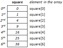
As an example, let's have a look at an integer array having 7 elements. The integer type elements of the array will all have the value of the square of their indexes (Figure I.15, “Graphical representation of an one-dimensional array”). It is a good solution to store the size of an array as a constant. According to what has been said so far, the definition of the array square is the following:
const int maxn =7;
int square[maxn];
In order to access the elements of the array in a linear order from its beginning to its end, we use in general a for loop, the variable of which stores the index of the array. (Normally, a correct for-loop runs from 0 to size minus one). Array elements are accessed by the indexing operator ([]).
for (int i = 0; i< maxn; i++)
    square[i] = i * i;
The size of memory in bytes allocated for the array square is returned by the expression sizeof (square), whereas the expression sizeof (square[0]) returns the size of one element. The number of elements of an array can therefore always be calculated by dividing the two elements by integer division:
int number_of_elements = sizeof(square) / sizeof(square[0]);
It should be noted that C++ carry out no check on array indexing. Trying to access an element at an index that is outside the array bounds can lead to runtime errors, and tracing back these errors can take too much time.
double october [31];
october [-1] = 0;    // error ↯
october [31] = 0;    // error ↯
In the following example, we calculate the average of float numbers read from the keyboard to an array of five elements, and then print out this average and the difference between each element and this average.
#include <iostream>
using namespace std;

const int maxn = 5 ;
int main()
{
    float numbers[maxn], average = 0.0;
    for (int i = 0; i <maxn; i++)
    {
        cout<<"numbers["<< i <<"] = ";
        cin>>numbers[i];        // reading from keyboard
        average += numbers[i];    // sum of all elements
    }
    cin.get();
    average /= maxn;            // counting the average
    cout<< endl << "The average is " << average << endl;

    // printing out differences
    for (int i = 0; i <maxn; i++) {
        cout<< i << ".\t" << numbers[i];
        cout<< '\t' << average-numbers[i] << endl;
    }
}
We should pay attention to how elements of an array are read from the keyboard. Array elements can only be accessed and set (from the keyboard) one by one.
numbers[0] = 12.23 numbers[1] = 10.2 numbers[2] = 7.29 numbers[3] = 11.3 numbers[4] = 12.7 The average is 10.744 0. 12.23 -1.486 1. 10.2 0.544001 2. 7.29 3.454 3. 11.3 -0.556 4. 12.7 -1.956 |
I.7.1.1.1. Initializing and assigning values to one-dimensional arrays
C++ language makes possible to give an initial value to array elements. When arrays are defined, the equal sign is followed by the values of the initialization list that are enclosed within curly brackets. These values are associated with the indexes of the array in that order:
element_typearray_name[size] = { initialization list delimited by commas };
Let's see some examples how to initialize vectors:
int primes[10] = { 2, 3, 5, 7, 11, 13, 17, 19, 23, 27 };

char name[8] = { 'I', 'v', 'a', 'n'};

double numbers[] = { 1.23, 2.34, 3.45, 4.56, 5.67 };
In the case of the array primes, we made sure that the number of elements in the list is equal to the size of the array. If the list contained more initial values than needed, compilers would send us an error message.
In the second example, the initialisation list contains less elements than the size of the array. In that case, the first four elements of the array name will have the given values, while the others will be 0. If we benefit from this possibility, we can easily set 0 for all elements of any array by:
int big[2012] = {0};
In the last example, the compiler sets the number of elements of the array numbers based on the number of constants provided in the initialisation list (5). This is a good solution if the number of elements is often changed between different compilations. In that case, the number of the elements can be obtained by the above mentioned method:
double numbers[] = { 1.23, 2.34, 3.45, 4.56, 5.67 };
const int numbers = sizeof(numbers) / sizeof(numbers[0]);
Initialisation lists may contain expressions the values of which are calculated runtime:
double eh[3]= { sqrt(2.3), exp(1.2), sin(3.14159265/4) };
For a more rapid but less secure management of arrays, the Standard Library functions declared in the cstring header file and beginning with ”mem” can also be used. The function memset () makes possible to set all elements of a char array to the same character or to set all elements of an array of any type to bytes with value 0:
char line[80];
memset( line, '=', 80 );
double balance[365];
memset( balance, 0, 365*sizeof(double) );
//or
memset( balance, 0, sizeof(balance) );
The latest example gives rise to the question what operations can be used in C++ for arrays besides the indexing and the sizeof operators. The response is easy: nothing. The reason for that is that C/C++ languages treat array names as constant value pointers that are set by compilers. We benefitted from that when we called memset () since the first parameter of the function should be a pointer.
There are two methods for value assignment between two arrays of the same type and size. In the first case, elements are copied from one to another in a for loop, in the second one, the Library function memcpy () is called.
#include <iostream>
#include <cstring>
using namespace std;

int main()
{
    const int maxn = 8 ;
    int source[maxn]= { 2, 10, 29, 7, 30, 11, 7, 12 };
    int destination[maxn];
    for (int i=0; i<maxn; i++) {
        destination[i] = source[i];    // copying elements
    }
    // or
    memcpy(destination, source, sizeof(destination));
}
memcpy () does not always function correctly if there is an overlap between source and destination, for example if only one part of an array has to be copied to free space for a new element. In that case as well, there are two possibilities: a for loop or the memmove () Standard Library function. In the following example, a new element is intended to be inserted in the array ordered at the position with index 1:
#include <iostream>
#include <cstring>
using namespace std;

int main()
{
    const int maxn = 10 ;
    int ordered[maxn]= { 2, 7, 12, 23, 29 };
    for (int i=5; i>1; i--) {
        ordered[i] = ordered[i-1];  // copying elements
    }
    ordered[1] = 3;
    // or
    memmove(ordered+2, ordered+1, 4*sizeof(int));
    ordered[1] = 3;
}
It should be noted that the address of the destination and source area is provided by using pointer arithmetic: ordered+2, ordered+1.
I.7.1.1.2. One-dimensional arrays and the typedef
As we have already mentioned, the readability of program code is increased if more complex type names are replaced by synonymous names. For that reason, typedef should be used for derived types.
Let's look an example where we aim at calculating the vector multiplication of two vectors of 3 integer elements and to place the new vector in a third vector. The general definition of vector multiplication:
|
| ||
|
|


The arrays necessary to solve the problem can be created in two ways:
int a[3], b[3], c[3];
or
typedef int vector3[3];
vector3 a, b, c;
The vectors a and b are initialized with constants:
typedef int vector3[3];
vector3 a = {1, 0, 0}, b = {0, 1, 0}, c;
c[0] =   a[1]*b[2] - a[2]*b[1];
c[1] = -(a[0]*b[2] - a[2]*b[0]);
c[2] =   a[0]*b[1] - a[1]*b[0];
typedef is also useful to reference an array containing 12 elements of type double with a pointer. The first idea should be to type
double *xp[12];
to create the type. When interpreting type expressions, the priority table of operators is useful (Appendix Section A.7, “Precedence and associativity of C++ operations”). On the basis of that, xp is an array of 12 elements and the array name is preceded by the type of its elements. That is why, xp is a pointer array with 12 elements. The order of the interpretation can be modified by parentheses:
double (*xp)[12];
In that case, xp is a pointer and the type of the referenced data is double[12], that is a double array of 12 elements. Now we are done! However, it is more rapid and safe to use the keyword typedef:
typedef double dvect12[12];
dvect12 *xp;
double a[12];
xp = &a;
(*xp)[0]=12.3;
cout << a[0];    // 12.3
I.7.1.2. Two-dimensional arrays
When scientific tasks are to be solved, it is often needed to store matrices in memory. For that purpose, the simplest form of multi-dimensional arrays has to be used, namely two-dimensional arrays:
element_typearray_name[size1][size2];
where sizes have to be specified by dimensions. As an example, let's store the following 3x4 matrix containing integers in a two-dimensional array.
|
|

In the definition, matrix elements can be given in many ways, we only have to make sure that the initialization list should contain the elements in the correct sequence.
int matrix[3][4] = { { 12, 23,  7, 29 },
                     { 11, 30, 12,  7 },
                     { 10,  2, 20, 12 } };
In order to access the elements of the array, we should use the indexing operator twice. The expression
matrix[1][2]
refers to the 2nd element of the 1st row (12). (It should be kept in mind that the first index is 0 in every dimension.)
On Figure I.16, “Graphical representation of a two-dimensional array”, the two-dimensional matrix array is represented with their row and column indexes (r/c).
The next program code searches for the biggest (maxe) and smallest (mine) element of the matrix above. In the solution there are nested for loops, generally used for the processing of two-dimensional arrays:
int maxe, mine;
maxe = mine = matrix[0][0];
for (int i = 0; i < 3; i++) {
    for (int j = 0; j < 4; j++) {
        if (matrix[i][j] > maxe )
             maxe = matrix[i][j];
        if (matrix[i][j] < mine )
             mine = matrix[i][j];
    }
}
Printing out two-dimensional arrays as a matrix is done by the following source code:
for (int i = 0; i < 3; i++) {
    for (int j = 0; j < 4; j++)
        cout<<'\t'<<matrix[i][j];
    cout<<endl;
}
I.7.1.3. Variable-length arrays
According to the previous C++ standard, arrays are created during compilation and for that purpose constant expressions defining their size are made use of. The C++11 standard (Visual C++ 2012) introduces the notion of variable-length arrays and therefore it extends the number of areas where they can be used. The variable-length array created during compilation can only have automatic lifetime, can only be local and cannot be defined with an initial value. Since these arrays can only be used in functions, it is possible that the size of these arrays are different each time the function is called - that is why they are called variable-length arrays.
The size of variable-length arrays can be provided by any integer type expression; however, the size cannot be modified after creation. Compilers apply the runtime version of the sizeof operator for variable-length arrays.
In the following example, the array is created only after its size is read from the keyboard:
#include <iostream>
using namespace std;

int main() {
    int size;
    cout << "The number of elements of the vector: ";
    cin >> size;
    int vector[size];
    for (int i=0; i<size; i++) {
        vector[i] = i*i;
    }
}
I.7.1.4. The relationship between pointers and arrays
In C++, there is a strong relation between pointers and arrays. Every operation that can be used with array indexing can also be carried out with pointers. One-dimensional arrays (vectors) and single indirection (”one-asterisked”) pointers are completely analogous with respect to form and content. The relationship between multi-dimensional arrays and multiple indirection pointers (having more asterisks) is only formal.
Let's see from where this strong relation between vectors and single indirection pointers comes from. Let's define a vector of five integer elements.
int a[5];
The elements of a vector are placed in memory in a linear sequence from a given address. All elements can be referenced by the form a[i] (Figure I.17, “The relationship between pointers and arrays”). Let's define a pointer p pointing to an integer, and then set it to point to the first element (to the 0th element) of the array, by the "address of" operator.
int *p;
p = &a[0];        or        p = a;
A pointer can be set by the name of the array since this is an int * type pointer that cannot be modified. (However, the statement p = &a; leads to a compilation error since the type of the right-hand side is int (*)[5].)
After these, if the variable *p - to which the pointer p points - is referenced, then it is actually the element a[0] that is accessed.
On the basis of the rules of pointer arithmetic, the addresses p+1, p+2 etc. refer the elements that follow the element to which p points. (It should be noted that elements preceding the variable can be adressed using negative numbers.) On the basis of that, every element of the array can be accessed by the expression *(p+i).
The role of the pointer p equals completely with that of the name of the array, since both define the beginning of the sequence of the elements. However, there is an important difference between the two pointers: pointer p is a variable (its value can therefore be modified any time), while a is a constant value pointer that the compiler fixes in memory.
Using the expressions of Figure I.17, “The relationship between pointers and arrays” the references figuring in the same row of the following table are identical:
|
|
The address of the ith element: | |||||
|
|
|
|
| |||
|
The 0th element of the array: | ||||||
|
|
|
|
|
|
| |
|
The ith element of the array: | ||||||
|
|
|
|
| |||
Most of C++ compilers transform all a[i] references automatically into *(a+i) and compiles this latter pointer form. However, this analogy is true in the inverse direction too, so instead of the indirection (*) operator, the indexing operator ([]) can always be used.
In the case of multi-dimensions, analogy is only formal; however, it can often help using correctly more complex data structures. Let's see the following double type matrix:
double m[2][3] = { { 10, 2, 4 },
                   { 7,  2, 9 } };
The rows of the array are placed in memory in a linear sequence. If the last dimension is left out, the pointer of the selected row is accessed: m[0], m[1], whereas the name of the array m points to the whole array (Figure I.18, “Two-dimensional arrays in memory”). It can be concluded from the above that two-dimensional arrays are actually vectors (one-dimensional arrays), the elements of which are vectors (pointers). Nevertheless, multi-dimensional arrays are always stored in a linear sequence in memory. In the previous example, the rows of the matrix given as initial value constitute the vectors from which the vector m is built up of.
The formal analogy between vectors and pointers makes it possible to rewrite indexing operators into indirection operators without a problem. All of the following expressions refer the same element of the two-dimensional array m (precisely 9):
m[1][2] *(m[1] + 2) *(*(m+1)+2)
I.7.2. Dynamically allocated arrays
A big quantity of data can be stored and processed easily and effectively with the help of arrays. However, the big disadvantage of traditional arrays is that their size is fixed during compilation and it is only during execution that we learn if too much memory was allocated. It is especially true for local arrays created within functions.
It is a general rule that only arrays of little size can be defined within functions. If a bigger quantity of data has to be stored, the methods for dynamic memory allocation should be used since there is much more space in the heap than in stack memory.
We should not forget that memory space can be allocated by the new operator not only for one but also for more elements standing one after the other. In that case, the allocated memory space can be freed by the delete[] operator.
Methods for dynamic memory allocation and deallocation are present in the form of functions in the Standard Library of C/C++. To access these functions, the cstdlib header file should be included in the source code. The malloc () function allocates a memory space of a given byte size and returns a pointer to the beginning of the block. The calloc () works in a similar way; however, the size of the memory block should be given in number of elements and element size, and it initializes the allocated memory block to zero. The realloc () resizes the already allocated memory block while keeping its original content (if a bigger is allocated). The free () deallocates the reserved memory block.
In case of objects, the new and delete operators should be used to access all relating operations.
I.7.2.1. One-dimensional dynamic arrays
It is one-dimensional dynamic arrays that are the most frequently used in programming.
type *pointer;
pointer = newtype [number_of_elements];
or
pointer = new (nothrow) type [number_of_elements];
The difference between the two methods can only be perceived if allocation has not been successful. In the first case, the compiler throws an exception ( bad_alloc ) if there is not enough available contiguous memory, and in the second case, a pointer with the value of 0 is returned.
In case of arrays, it is extremely important not to forget about deleting allocated memory:
delete [] pointer;
In the following example, the user is asked to enter the array size. Then a memory block is allocated for the array and finally it is filled up with random numbers.
#include <iostream>
#include <exception>
#include <ctime>
#include <cstdlib>
using namespace std;

int main() {
   long *data, size;
   cout << "\nEnter the array size: ";
   cin >> size;
   cin.get();

   // Memory allocation
   try {
     data = new long [size];
   }
   catch (bad_alloc) {
      // Unsuccessful allocation
      cerr << "\nThere is not enough memory!\n" << endl;
      return -1;  // Program is exited
   }
   // Filling up the array with random numbers
   srand(unsigned(time(0)));
   for (int i=0; i<size; i++) {
       data[i] = rand() % 2012;
       // or  *(data+i) = rand() %2012;
   }
   // Deleting (freeing) allocated memory space
   delete[] data;
   return 0;
}
I.7.2.2. Two-dimensional dynamic arrays
We have already mentioned in the previous subchapters that two-dimensional arrays are actually vectors of one-dimensional vectors (rows). As a consequence, a two-dimensional array of any size cannot be created at runtime since compiler has to know the type (the size) of the elements (the row vectors). However, the number of the elements (the rows) can be provided later. The new in the following example returns a pointer to the created two-dimensional array.
const int rowlength = 4;
int number_of_rows;
cout<<"Number of rows: "; cin >> number_of_rows;
int (*mp)[rowlength] = new int [number_of_rows][rowlength];
The solution becomes much more understandable if the keyword typedef is used:
const int rowlength = 4;
int number_of_rows;
cout<<"Number of rows: "; cin >> number_of_rows;
typedef int rowtype[rowlength];
rowtype *mp = new rowtype [number_of_rows];
For both solutions, setting all elements to zero can be carried out by the following loops:
for (int i=0; i<number_of_rows; i++)
    for (int j=0; j<rowlength; j++)
        mp[i][j]=0;
where mp[i] refers to the ith row, and mp[i][j] refers to the jth element of the ith row. If the former statements are placed within the main () function, the mp pointer is placed in stack while the whole two-dimensional array in the heap. This solution has two drawbacks: arrays need memory space on the first hand, and it is annoying to provide the length of rows compile-time on the other hand.
Let's see how to avoid the constraints of memory and those of fixed row length. The next two solutions are based on the idea that arrays can be made from pointers.
In the first case, the pointer array fixing the number of rows is created in the stack and it is only row vectors that are created dynamically (Figure I.19, “Dynamically allocated row vectors”).
The pointer vector of 3 elements that selects the rows:
int* ps[3]= {0};The dynamic creation of rows, if rows have 4 elements:
for (int i=0; i<3; i++)
    ps[i] = new int[4];
Elements can be accessed by the operators * and []:
*(ps[1] + 2) = 123;
cout << ps[1][2];
Finally, we should not forget about freeing the dynamically allocated memory blocks.
for (int i=0; i<3; i++)
    delete[] ps[i];
If the number of rows and columns are to be set runtime, the pointer array of the previous example should be defined dynamically. In that case, stack only contains one pointer of type int * (Figure I.20, “Dynamically allocated pointer vector and row vectors”).
Memory allocation, access and deallocation can easily be traced in the following example code:
#include <iostream>
using namespace std;

int main() {
    int number_of_rows, rowlength;
    cout<<"Number of rows: "; cin >> number_of_rows;
    cout<<"The length of rows: "; cin >> rowlength;

    // Memory allocation
    int* *pps;
    // Defining the pointer vector
    pps = new int* [number_of_rows];

    // Allocating rows
    for (int i=0; i<number_of_rows; i++)
        pps[i] = new int [rowlength];

    // Accessing the array
    for (int i=0; i<number_of_rows; i++)
        for (int j=0; j<rowlength; j++)
            pps[i][j]=0;

    // Deleting (freeing) allocated memory space
    for (int i=0; i<number_of_rows; i++)
        delete pps[i];
    delete pps;
}
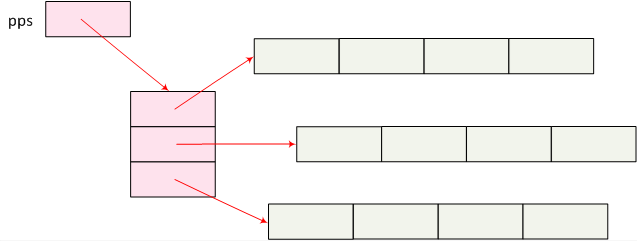
I.7.3. The usage of the vector type
Nowadays, C++ source codes use more and more frequently the vector type of C++ Standard Library (STL) instead of traditional one- or two-dimensional arrays. This type has all the features (resizing, checking that the provided index is within boundaries, automatic memory deallocation) needed for a secure usage of arrays.
Contrary to the already discussed types, vector type is parameterizable, which means that the type of stored elements should be provided within <> signs after the word vector . The created vectors, similarly to the cout and cin objects, are also objects that have their own operations and functions.
I.7.3.1. One-dimensional arrays in vectors
As its name suggests, vector type replaces one-dimensional arrays. Instead of presenting all features of that type, we will only concentrate on some basic useful information.
Let's see a solution for defining vectors, which needs that the vector header file be included in the source code.
vector<int> ivector;
ivector.resize(10);

vector<long> lvector(12);
vector<float> fvector(7, 1.0);
ivector is an empty vector, the size of which is set by the function resize () to 10. lvector contains 12 elements of type long. In both cases, all elements are initialized to 0. fvector is created with 7 elements of type float, the values of which are all initialized to 1.0.
The actual number of elements can be obtained by the function size (), accessing elements is possible by the traditional indexing operator. An important feature of vector type is the function push_back () that adds an element to the vector.
#include <iostream>
#include <vector>
using namespace std;

int main() {
    vector<int> ivector(10, 5);

    ivector.push_back(10);
    ivector.push_back(2);

    for (unsigned index=0; index<ivector.size(); index++) {
        cout << ivector[index] << endl;
    }
}
It should be noted that STL data containers can be managed completely with predefined algorithms ( algorithm header file).
I.7.3.2. Two-dimensional arrays in vectors
Two-dimensional, dynamic arrays can be created by nesting vector types, and it is much easier than the methods mentioned before.
#include <iostream>
#include <vector>
using namespace std;

int main() {
    int number_of_rows, rowlength;
    cout<<"Number of rows: "; cin >> number_of_rows;
    cout<<"The length of rows: "; cin >> rowlength;

    vector< vector<int> > m (number_of_rows, rowlength);

    // Accessing the array
    for (int i=0; i<number_of_rows; i++)
        for (int j=0; j<rowlength; j++)
            m[i][j]= i+j;
}
I.7.4. Handling C-style strings
The primitive types of C/C++ do not contain the string type appropriate for storing character sequences. But since it is indispensable to store and to process strings in C/C++ programs, storage can be realised by one-dimensional character arrays. For string processing, it is also needed that valuable characters are always closed by a byte with value 0. There are no operators for managing strings; however, there are many functions for that purpose (in the cstring header file).
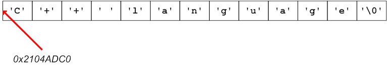
In program codes, we often use texts enclosed within quotation marks (string literals), that compilers store among the initialized data according to the things said before.
cout << "C++ language";
When interpreting the statement above, the string is copied into memory, (Figure I.21, “String constant in memory”) and as a right operand of the operation << , an address of type const char * is compiled. When the program is executed, the cout object prints out character by character the content of the selected memory block until it reaches the byte with value 0.
Strings composed of wide characters are also stored in that way but in this case the type of the elements of the array is wchar_t.
wcout << L"C++ language";
In C++, the types string and wstring can also be used to process texts, so we give an overview of these types, too.
I.7.4.1. Strings in one-dimensional arrays
When memory space is allocated for a character string, the byte indicating the end of the string should also be taken into consideration. If a text of at most 80 characters is intended to be stored in the array named str then its size should be 80+1=81:
char line[81];
In programming tasks, we often use strings having an initial value. In order to provide an initial value, we can use the solutions already presented in relation with arrays; however, we should not forget about the final '\0' character:
char st1[10] = { 'O', 'm', 'e', 'g', 'a', '\0' };

wchar_t wst1[10] = { L'O', L'm', L'e', L'g', L'a', L'\0' };

char st2[] = { 'O', 'm', 'e', 'g', 'a', '\0' };

wchar_t wst2[] = { L'O', L'm', L'e', L'g', L'a', L'\0' };
Compiler allocates 10 bytes of memory for the string st1 and the given characters are copied into the first 6 bytes. However, st2 will be of a size of as many bytes as many characters are provided in the initialization list. For the wst1 and wst2 wide character strings, compilers allocate a memory space twice as much (in bytes) as in the previous ones.
Initializing character arrays is much safer by using string literals (string constants):
char st1[10] = "Omega";    wchar_t wst1[10] = L"Omega";

char st2[] = "Omega";        wchar_t wst2[] = L"Omega";
Whereas the initialization have the same results in both cases (i.e. with characters and with string constants), using string constants is easier to understand. Not to mention the fact that the 0 byte closing strings is placed in memory by the compiler.
The result of the storage in arrays is that there is no operation available in C++ for strings either (value assignment, comparison etc.). However, there are many Library functions for processing character sequences. Let's see some basic functions processing character sequences.
|
Operation |
Function (char) |
Function (wchar_t) |
|---|---|---|
|
reading text from the keyboard |
cin >>, cin . get (), cin . getline () |
wcin >>, wcin . get (), wcin . getline () |
|
printing out a text |
cout << |
wcout << |
|
value assignment |
strcpy (), strncpy () |
wcscpy(), wcsncpy() |
|
concatenation |
strcat (), strncat () |
wcscat(), wcsncat() |
|
getting the length of a string |
strlen () |
wcslen() |
|
comparison of strings |
strcmp (), strcnmp () |
wcscmp(), wcsncmp() |
|
searching for a character in a string |
strchr () |
wcschr() |
In order to manage strings with char type characters, we need to include the iostream and cstring header files, whereas wide character functions are found in cwchar .
The following example code transforms the text read from the keyboard and prints out all its characters in capital letters and in reverse order. It can clearly be seen from the example that we should use both Library functions and character array notion to efficiently manage strings.
#include <iostream>
#include <cstring>
#include <cctype>
using namespace std;

int main() {
   char s[80];
   cout <<"Type in a text: ";
   cin.get(s, 80);
   cout<<"The read text: "<< s << endl;
   for (int i = strlen(s)-1; i >= 0; i--)
      cout<<(char)toupper(s[i]);
   cout<<endl;
}
The wide character version of the previous solution is:
#include <iostream>
#include <cwchar>
#include <cwctype>
using namespace std;

int main() {
   wchar_t s[80];
   wcout <<L"Type a text: ";
   wcin.get(s, 80);
   wcout<<L"The read text: "<< s << endl;
   for (int i = wcslen(s)-1; i >= 0; i--)
      wcout<<(wchar_t)towupper(s[i]);
   wcout<<endl;
}
In both examples, we used the secure cin . get () function to read a text from the input. The function reads all characters until <Enter> is pressed. However, the given array can only have a number of characters same as or less than size-1, which is provided as one of its argument.
I.7.4.2. Strings and pointers
Character arrays and character pointers can both be used to manage strings but pointers should be used more carefully. Let's see the following frequent definitions.
char str[16] = "alfa";

char *pstr = "gamma";
In the first case, the compiler creates the array str of 16 elements and then it copies in the characters of the provided initial value and the byte with value 0. In the second case, the compiler stores the initial text in the area reserved for string literals, then it initializes the pointer pstr to the beginning address of the string.
The value of the pointer pstr can be modified later (which causes the loss of the string "gamma"):
pstr = "iota";
A pointer value assignment takes place here since pstr now points to the address of the new string literal. On the contrary, if it is the name of the array str to which a value is assigned, an error message is obtained:
str = "iota"; // error! ↯
If a string has to be processed character by character, then we can choose from the array and the pointer approach. In the following example code, the read character sequence is first encrypted with the exclusive-or operation and then its content will be replaced again by its original content. (During encryption the string is treated as an array, and during decryption the pointer approach is used.) In both cases, the loop ends if the string closing zero byte is reached.
#include <iostream>
using namespace std;

const unsigned char key = 0xCD;
int main() {
    char s[80], *p;
    cout <<"Type in a text: ";
    cin.get(s, 80);

    for (int i = 0; s[i]; i++)            // encryption
        s[i] ^= key;
    cout << "The encrypted text: "<< s << endl;

    p = s;
    while (*p)                         // decryption
        *p++ ^= key;
    cout << "The original text: "<< s << endl;
}
In the following example, the increment and indirection operators are used together, which requires more carefulness. In the following example, the pointer sp points to a dynamically stored character sequence. (It should be noted that most C++ implementations do not allow modifications of string literals.)
char *sp = new char [33];
strcpy(sp, "C++");
cout << ++*sp << endl;        // D
cout << sp << endl;        // D++
cout << *sp++ << endl;        // D
cout << sp << endl;        // ++
In the first case (++*sp), the compiler interprets first the indirection operator and then increments the referred charater. In the second case (*sp++), the compiler first steps the pointer to the next character but since it is a post-increment operator, increment takes place after processing the whole expression. The value of the expression is the referenced character.
I.7.4.3. Using string arrays
Most C++ programs contain texts (e.g. error messages) that are printed on the basis of a certain index (error code). The simplest solution for storing such texts is defining string arrays.
When string arrays are planned, it should be decided whether they will be two-dimensional or pointer arrays. For beginners in C++ programming, it is often difficult to differentiate between the two. Let's see the following two definitions.
int a[4][6];
int* b[4];
a is a "real” two-dimensional array for which the compiler allocates a continuous memory block for 24 (4x6) elements of type int. On the contrary, b is a pointer vector of 4 elements. The compiler allocates space for only four pointers based on this definition. The other parts of initialization is done later in the code. Let's initialize the pointer array so that it would be able to store 5x10 integer elements.
int s1[6], s2[6], s3[6], s4[6];
int* b[4] = { s1, s2, s3, s4 };
It is clear that besides the memory block needed for 24 int elements, further memory space was also used (for the pointers). At this point, it would be logical to ask what the advantages are of using pointer arrays. The response can be found in the length of rows. While in a two-dimensional array every row contains the same number of elements,
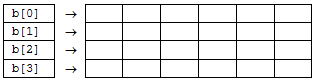
the size of each row can be different in pointer arrays.
int s1[1], s2[3], s3[2], s4[6];
int* b[4] = { s1, s2, s3, s4 };
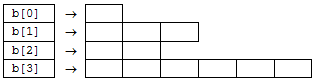
The other advantage of pointer arrays is that their structure is in line with the possibilities of dynamic memory allocation, thus it has an important role when dynamically allocated arrays are to be created.
After this short introduction, let's see the subject of the present subchapter: the creation of string arrays. In general, string arrays are defined by providing them initial values. In the first example, a two-dimensional array is defined with the following statement:
static char names1[][10] = { "Ivan",
                             "Olesya",
                             "Anna",
                             "Adrienn" };
This definition results in the creation of a 4x10 character array: the number of the rows is determined by the compiler on the basis of the initialization list. The rows of the two-dimensional character array are placed in a linear sequence in memory (Figure I.22, “String array stored in a two-dimensional array”).
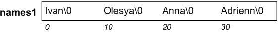
In the second case, a pointer array is used to store the addresses of the names:
static char* names2[] = { "Ivan",
                          "Olesya",
                          "Anna",
                          "Adrienn" };
The compiler allocates four blocks of different size in memory, as it is shown on Figure I.23, “Optimally stored string array”:
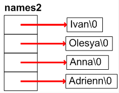
It is worth comparing the two solutions with respect to definition and memory access.
cout << names1[0] << endl;        // Ivan
cout << names1[1][4] << endl;    // y
cout << names2[0] << endl;        // Ivan
cout << names2[1][4] << endl;    // y
I.7.5. The string type
In the C++ Standard Template Library (STL), there are classes that support string management. The solutions presented above are useful for C-style character sequences. Now let's learn the features of the types string and wstring.
In order to access C++ style character sequence management, it is necessary to include the string header file in the source code. If string objects are defined as type string, many comfortable string processing operations can be carried out with the help of operators and member functions. Let's see some of them. (In the table, member functions are preceded by a point. The name of a member function is provided after the name of the object and is separated from that by a dot.) In order to process wide character strings, we need not only the string header file but also the cwchar file.
|
Operation |
C++ solution - string |
C++ solution - wstring |
|---|---|---|
|
reading text from the keyboard |
cin>> , getline () |
wcin>> , getline () |
|
printing out a text |
cout<< |
wcout<< |
|
value assignment |
= , .assign () |
= , .assign () |
|
concatenation |
+ , += |
+ , += |
|
accessing the characters of a string |
[] |
[] |
|
getting the length of a string |
.size () |
.size () |
|
comparison of strings |
.compare (), == , != , < , <= , > , >= |
.compare (), == , != , < , <= , > , >= |
|
conversion into C-style character sequence |
.c_str (), .data () |
.c_str (), .data () |
Let's rewrite our encrypting program by using C++ style string processing.
#include <string>
#include <iostream>
using namespace std;

const unsigned char key = 0xCD;
int main() {
    string s;
    char *p;
    cout <<"Type in a text   : ";
    getline(cin, s);

    for (int i = 0; s[i]; i++)     // encryption
        s[i] ^= key;
    cout << "The encrypted text: "<< s << endl;

    p=(char *)s.c_str();
    while (*p)                    // decryption
        *p++ ^= key;
    cout << "The original text: "<< s << endl;
}
The solution of the task with wide character strings (wstring) can be found in the following code:
#include <string>
#include <iostream>
#include <cwchar>
using namespace std;

const unsigned wchar_t key = 0xCD;
int main()
{
    wstring s;
    wchar_t *p;
    wcout <<L"Type a text  : ";
    getline(wcin, s);

    for (int i = 0; s[i]; i++)     // encryption
        s[i] ^= key;
    wcout<<L"The encrypted text: "<< s << endl;

    p=(wchar_t *)s.c_str();
    while (*p)                    // decryption
        *p++ ^= key;
    wcout<<L"The original text: "<<s<<endl;
}
I.8. User-defined data types
Arrays can store and process easily a set of data of the same type. However, most programming tasks require treating data of different types logically as one unit. In C++, there are many possibilities for that among which the most important ones are structures and classes since they provide the basis for the object-oriented solutions discussed in Chapter III, Object-oriented programming in C++ of the present book.
In the following, we will learn more about structure, class, bit fields and union types from among the aggregate types. In this chapter, stress will be laid more on structures (structs). The reason for that is that all notions and solutions related to structures can be used for other user-defined types without exception.
I.8.1. The structure type
In C++, a structure (struct) is a type that is a set of many data of any type (except for void and function types). These data members that are traditionally called structure elements or data members, have names that are only valid within their structure. (In other languages, the notion field is used for these elements; however, in C++, this name is attached to bit structures.)
I.8.1.1. Structure type and structure variables
A variable of a structure type can be created in two steps. First, a structure type has to be declared and then variables can be defined. The general declaration of structures is as follows:
struct structure_type {
type 1 member 1 ; // without an initial value!
type 2 member 2 ;
. . .
type n member n ;
};
It should be noted that the curly brackets enclosing structure declarations have to be followed by a semicolon. Data members should be declared according to the standard variable declaration rules of C++; however, initial values cannot be given for them. A structure variable (a structure) of the type above can be created by the already known method:
struct structure_type structure_variable; // C/C++
structure_type structure_variable; // only in C++
In C++, the name standing after the keywords struct, union and class can be used as type names without using the keywords. When typedef is used, the difference between the two programming languages disappears:
typedef struct {
type 1 member 1 ;
type 2 member 2 ;
. . .
type n member n ;
} structure_type;
structure_type structure_variable; // C/C++
Similarly to those of arrays, the definitions of structure variables may contain initial values. The lists of the expressions, separated from one another by commas, initializing the data members should be enclosed within curly brackets.
structure_type structure_variable= {initial_value_list}; // C/C++
It should be noted that most software development companies support structure definitions with typedef in order that confusions be avoided.
It should be noted that the visibility of member names within a struct is limited to the structure. This means that the same name can be used within the given visibility level (module, block), in other structures or as independent variable names:
struct s1 {
    int a;
    double b;
};

struct s2 {
    char a[7];
    s1 b;
};

long a;
double b[12];
Let's see an example for defining a structure type. The following data structure can be useful for a software cataloguing music CDs:
struct musicCD {
       // the performer and the title of the CD
       string performer, title;
       int year;            // year of publication
       int price;        // price of the CD
};
Variables can be defined with the type musicCD:
musicCD classic = {"Vivaldi","The Four Seasons", 2009, 2590};
musicCD *pmusic = 0, rock, tale = {};
From the structure type variables above, rock is not initialised whereas all members of the structure tale will have the default initial value corresponding to their type. The pointer pmusic does not refer to any structure.
We created a new user-defined type by having declared the structure. The data members of the variable of a structure type are stored in memory in the order of their declaration. On Figure I.24, “Structure in memory” , we can see the graphical layout of the data structure created by the definition
musicCD relax;
It can be clearly seen from the figure that the names of the data members indicate their distance from the beginning of the structure. In general, the size of a structure is equal to the sum of the sizes of its data members. However, in some cases, "holes" may appear between the members of a structure (when speed is optimized or when members are aligned to memory boundaries etc.). But it is always the punctual value that is obtained by the sizeof operator.
In most cases, the compiler is entrusted with the alignment of data members to memory boundaries. For a rapid access, it places the data by optimizing storage to the given hardware. However, if structures are exchanged by files between different platforms, the alignment used for saving has to be set in the reader program.
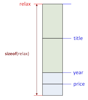
In order to control the C++ compilers, we use the preprocessor directive #pragma, the features of which are completely implementation-dependent. For example, in Visual C++, the alignment to a byte boundary is done by the following directive, which has to be placed before the structure definition:
#pragma pack(1)
The argument of pack can be 1, 2, 4, 8 or 16. Without arguments, Visual C++ uses the default value for 32-bit systems: 4. Let's see the effects of the directive in the case of the following structure type.
#pragma pack(alignment)
struct mix {
    char ch1, ch2, ch3;
    short sh1, sh2;
    int n;
    double d;
};
#pragma pack()
I.8.1.2. Accessing the data members of structures
The word structure is often used alone but in that case it means a variable created by a given structure type and not the type. Let's define some variables by using the type musicCD declared before.
musicCD s1, s2, *ps;
The memory space necessary for storing the variables s1 and s2 of type musicCD is allocated by the compiler. In order to be able to access the structure with the pointer ps of type musicCD, we have two possibilities. In the first case, ps is simply redirected to the structure s1:
ps = &s1;
The other possibility is to use dynamic memory allocation. In the following example code, memory is reserved for the structure musicCD, than it is deallocated:
ps = new (nothrow) musicCD;
if (!ps) exit(-1);
// ...
delete ps;
After providing the appropriate definitions, we have three structures: s1, s2 and *ps. Let's see how to give values to data members. In C++, it is done by the dot ( . ) operator. The left-hand side operand of dot operators is a structure variable, the right-hand side operand selects a data member within the structure.
s1.performer = "Vivaldi";
s1.title    = "The Four Seasons";
s1.year     = 2005;
s1.price     = 2560;
If the dot operator is used on a structure to which ps points, precedence rules make it obligatory to enclose within parentheses the expression *ps:
(*ps).performer = "Vivaldi";
(*ps).title    = "The Four Seasons";
(*ps).year     = 2005;
(*ps).price     = 2560;
Since in C++, we often use structures to which a pointer points, this programming language reserves an independent operator, more precisely the arrow operator (->), for referencing data members. (The arrow operator consists of two characters: a minus and a greater than sign.) Arrow operators make more readable value assignments for data members of a structure to which ps points to:
ps->performer = "Vivaldi";
ps->title    = "The Four Seasons";
ps->year     = 2005;
ps->price     = 2560;
The left-hand operand of arrow operators is the pointer to a structure variable, whereas the right-hand operand selects the data member within that structure, similarly to dot operators. Accordingly, the meaning of the expression ps->price is: "the data member named price within the structure to which the pointer ps points".
We recommend that dot operators should be used only for direct references (accessing a data member of a variable of structure type) while arrow operators should be used only for indirect references (accessing a data member of the structure to which a pointer points).
A special case of structure value assignment is when the content of a structure type variable is intended to be assigned to another variable of the same type. This operation can even be carried out by data members:
s2.performer = s1.performer;
s2.title     = s1.title;
s2.year      = s1.year;
s2.price     = s1.price;
however, C++ can also interpret the assignment operator (=), so it can be used for structure variables:
s2  = s1 ;  // this corresponds to the 4 assignments above
*ps = s2 ;
s1  = *ps = s2 ;
This way of value assignment simply means copying the memory block occupied by the structure. However, this operation results in a problem if the structure contains a pointer that refers to an external memory space. In that case, it is programmers that have to solve this problem by assigning values for each data member one by one or the other possibility is to overload the copy operation (operator overloading) by creating an assignment operator (see Chapter III, Object-oriented programming in C++) for the structure.
Structures are accessed by data members during data input/output operations. The following example code reads the structure musicCD by asking the user to type them in and then prints out the entered data:
#include <iostream>
#include <string>
using namespace std;

struct musicCD {
       string performer, title;
       int year, price;
};

int main() {

   musicCD cd;

   // reading the data from the keyboard
   cout<<"Please type in the data of the music CD." << endl;
   cout<<"Performer           : ";    getline(cin, cd.performer);
   cout<<"Title               : ";    getline(cin, cd.title);
   cout<<"Year of publication : ";    cin>>cd.year;
   cout<<"Price               : ";    cin>>cd.price;
   cin.get();

   // printing out the data
   cout<<"\nData of the music CD:" << endl;
   cout<<"Performer           : ";    cout << cd.performer << endl;
   cout<<"Title               : ";    cout << cd.title << endl;
   cout<<"Year of publication : ";    cout << cd.year << endl;
   cout<<"Price               : ";    cout << cd.price << endl;
}
I.8.1.3. Nested structures
As we have already said, structures can have data members of any type. If a structure has one or more data members that are also structures, it is a nested structure.
Let's suppose that some personal data are intended to be stored in a structure. Among personal data, a separate structure is defined for dates:
struct date {
    int year, month, day;
};

struct person {
    string name;
    date birthday;
};
Let's create two persons in the following way: the first one will be initialized by an initialization list, and let's assign values separately to the members for the other one.
person brother = { "Ivan", {2004, 10, 2} };
person student;

student.name = "Bill King";
student.birthday.year = 1990;
student.birthday.month = 10;
student.birthday.day = 20;
In the initialization list, constants initializing inner structure do not necessarily have to be enclosed within curly brackets. In the second case, student.birthday refers the structure birthday of the structure student. This is followed by the dot operator (.) and the name of a data member of the inner structure.
If the structure of type date is not used anywhere else then it can be integrated directly as an anonymous structure in the structure person:
struct person {
    string name;
    struct {
        int year, month day;
    } birthday;
};
When creating more complex dynamic data structures (e.g. linear lists), elements of a given type have to be concatenated into a chain. Elements of this kind contain some kind of data and a pointer in general. C++ makes it possible to define a pointer with the type of the structure to be declared. These structures, which contain a pointer to themselves as a data member, are called self-referential structures. As an example, let's see the declaration of list_element.
struct list_element {
      double data_member;
      list_element *link;
};
This recursive declaration makes it possible that the pointer link points to the structure of type list_element. The declaration above does not nest the two structures in each other since the structure which we will reference later with the pointer will be placed somewhere else in memory. However, C++ compilers need this declaration in order to be able to allocate memory in compliance with the declaration, that is to get to know the size of the variable to be created. The declaration above makes compilers allocate for the pointer memory space the size of which is independent of that of the structure.
I.8.1.4. Structures and arrays
Programming can be made much more efficient if arrays and structures are used together in one data type. In the following simple codes, we first place a one-dimensional array within a structure then we create a one-dimensional array of structure type elements.
I.8.1.4.1. Arrays as data members of a structure
In the following example, besides an integer vector (v), we also store the number of valuable elements (n) in the structure svector:
const int maxn = 10;
struct svector {
    int v[maxn];
    int n;
};

svector a = {{23, 7, 12}, 3};
svector b = {{0}, maxn};
svector c = {};

int sum=0;
for (int i=0; i<a.n; i++) {
    sum += a.v[i];
}

c = a;
In the expression a.v[i], there is no need to use parentheses since the two operations has the same precedence so the expression is evaluated from left to right. So first the member v is selected from the structure a, then the ith element of the array a.v is accessed. Another interesting part of the solution is that the elements of the vector are also copied from one of the structures to another when value assignment takes place between the two structures.
The structure of type svector can also be created dynamically. However, in that case, the structure should be accessed by an arrow operator.
svector *p = new svector;
p->v[0] =  2;
p->v[1] = 10;
p->n    =  2;
delete p;
I.8.1.4.2. Structures as array elements
A structure array has to be defined exactly in the same way as arrays of any other type. As an example, let's make use of the type musicCD declared above to create a CD-catalogue of 100 elements and let's give initial values for the first two elements of CDcatalog.
musicCD CDcatalog[100]={{"Vivaldi","The Four Seasons",2004,1002},{} };
In order to reference the data members of structures as array elements, we have to first select the array element and then the structure member:
CDcatalog[10].price = 2004;
If the CD-catalogue is intended to be created dynamically, identification has to be done with a pointer:
musicCD *pCDcatalog;
Memory space for structure elements can be allocated by the operator new in the dynamically managed memory space:
pCDcatalog = new musicCD[100];
The structure stored in an array element can be accessed by using the dot operator:
pCDcatalog[10].price = 2004;
If array elements are not needed anymore, then the allocated memory space should be freed by the operator delete []:
delete[] pCDcatalog;
Certain operations (like sorting) can be carried out more efficiently if the pointers of the dynamically created CDs are stored in a pointer array:
musicCD* dCDcatalog[100];
The following loop allocates space for the structures in the dynamically managed memory:
for (int i=0; i<100; i++)
  dCDcatalog[i] = new musicCD;
Then, the structures selected by the array elements can be referenced by the arrow operator:
dCDcatalog[10]->price = 2004;
If these structures are not needed anymore, then we should iterate through the elements and delete them from the memory space:
for (int i = 0; i < 100; i++)
   delete dCDcatalog[i];
The following example searches for all CDs published between 2010 and 2012 in a dynamically created CD catalogue containing a fix number of CDs.
#include <iostream>
#include <string>
using namespace std;

struct musicCD {
    string performer, title;
    int year, price;
};

int main() {
    cout<<"The number of CDs:";
    int num;
    cin>>num;
    cin.ignore(80, '\n');

    // Memory allocation with checking
    musicCD *pCDcatalog = new (nothrow) musicCD[num];
    if (!pCDcatalog) {
        cerr<<"\a\nThere is not enough memory!\n";
        return -1;
    }

    // Reading the data of CDs from the keyboard
    for (int i=0; i<num; i++) {
        cout<<endl<<"The data of the "<<i<<"th CD:"<<endl;
        cout<<"Performer: ";
                   getline(cin, pCDcatalog[i].performer);
        cout<<"Title:    "; getline(cin, pCDcatalog[i].title);
        cout<<"Year:     "; cin>>pCDcatalog[i].year;
        cout<<"Price:     "; cin>>pCDcatalog[i].price;
        cin.ignore(80, '\n');
    }

    // Searching for the requested CDs
    int found = 0;
    for (int i = 0; i < num; i++) {
        if (pCDcatalog[i].year >= 2010 &&
                pCDcatalog[i].year <= 2012) {
            cout<<endl<<pCDcatalog[i].performer<<endl;
            cout<<pCDcatalog[i].title<<endl;
cout<<pCDcatalog[i].year<<endl;
            found++;
        }
    }

    // Printing out the results
    if (found)
        cout<<"\nThe number of found elements: "<<found<<endl;
    else
        cout<<"There is no CD that matches the criteria!"<<endl;

    // Deallocating memory space
    delete [] pCDcatalog;
}
This program is interactive, that is data should be provided by a user, and prints out results on the screen. Testing with a bigger amount of data is more difficult in that way.
However, most operating systems make it possible to redirect the standard input and output of a program to a file. For that purpose, the input data should be typed in a file exactly in the same way the program expects them (e.g. CDs.txt), and this file name should be provided after a lower than sign when the program (CDCatalogue) is executed from the command line:
CDCatalogue <CDs.txt

CDCatalogue <CDs.txt >Results.txt
The second command writes the results to a separate file (Figure I.25, “Processing data in the program CDCatalogue”). (In the development environment of Visual C++ , the redirection properties can be set in the window Project /project Properties , on the tab named Debugging , in the line of Command Arguments .)
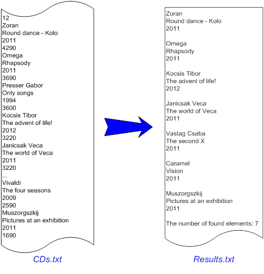
I.8.1.5. Creating singly linked lists
The simplest forms of linked lists are singly linked lists in which all elements possess a reference to the next list element. The reference in the last element has the value null (Figure I.26, “A singly linked list”).
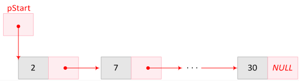
The list is selected in the memory by the pointer pStart so the value of the latter should always be kept. If the value of pStart is set to another value, the list becomes inaccessible.
Let's see what advantages the usage of a linear list has as compared with vectors (one-dimensional arrays). The size of a vector is fixed when it is defined; however, the size of a list can be increased or decreased dynamically. There is also an important difference between the two how elements are inserted in or removed from them. Whereas these operations only require the copy of some pointers in the case of lists, these operations require moving a big amount of data in vectors. There is also a significant difference between the two with respect to the structure of the storage unit, that is that of the element:
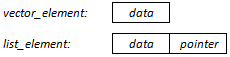
Vector elements only contain the stored data whereas list elements also contain a reference (a pointer) to (an)other element(s). C++ list elements can be created by the already presented self-referential structure.
As an example, let's store integer numbers in a linear list, the elements of which have the following type:
struct list_element {
    int data;
    list_element *pnext;
};
Since we allocate memory for each new list element in this example, this operation is carried out by a function to be presented in the next chapter of the present book:
list_element *NewElement(int data) {
    list_element *p = new (nothrow) list_element;
    assert(p);
    p->data = data;
    p->pnext = NULL;
    return p;
}
That function returns the pointer of the new list element and initializes it if this function has run with success. We should not forget about calling the function assert (). This macro interrupts running the program and prints out the message "Assertion failed: p, file c:\temp\list.cpp, line 16” if its argument has the value of 0.
When created, the list is filled up by the elements of the following array:
int data [] = {2, 7, 10, 12, 23, 29, 30};
const int num_of_elements = sizeof(data)/sizeof(data[0]);
For a successful management of the list, we need additional variables and the pointer pStart to the beginning of the list:
list_element *pStart = NULL, *pActual, *pPrev, *pNext;
When we are dealing with a given element (pActual) of the list, we might need to know where the preceding element (pPrev) and the next one (pNext) are. In this example, in order to facilitate our task we hypothesise that the list always exists when it has been created, that is the pointer pStart is never null.
Creating the list and filling up it from the array data. When a list is created, there are three separate tasks to carry out with each element:
memory allocation (with checking if it has taken place) for a new list element (NewElement()),
assigning data to the list element (NewElement()),
adding the list element to (the end of) the list. When an element is added to a list, the things to be done are different in the case of first and non-first elements.
for (int index = 0; index<num_of_elements; index++) {
    pNext = NewElement(data[index]);
    if (pStart==NULL)
       pActual = pStart = pNext ;        // first element
    else
       pActual = pActual->pnext = pNext;    // not a first element
}
pActual->pnext = NULL;    // closing the list
// list: pStart ➝ 2 ➝ 7 ➝ 10 ➝ 12 ➝ 23 ➝ 29 ➝ 30
When printing out the elements of the list, we start from the pointer pStart and step to the next element in a loop until the null pointer indicating the end of the list is reached:
pActual = pStart;
while (pActual != NULL) {
    cout<< pActual->data << endl;
    // stepping to the next element
    pActual = pActual->pnext;
}
It is often needed to remove an element from a list. In the following example, the list element to be removed is identified by its index (Indexing starts with 0 from the element to which the pointer pStart points to. This example code is not able to remove the 0th and the last element!) The removal operation also consists of three steps:
// identifying the place of the element having the index 4 (23)
pActual = pStart;
for (int index = 0; index<4; index++) {
    pPrev    = pActual;
    pActual = pActual->pnext;
}
// removing the element of the linked list
pPrev->pnext = pActual->pnext;
// deallocating memory space
delete pActual;
// the list: pStart ➝ 2 ➝ 7 ➝ 10 ➝ 12 ➝ 29 ➝ 30
When the 0th element is removed, the pointer pStart has to be set to pStart->pnext before removal. When it is the last element that is removed, the member pnext of the element immediately before the last one has to be set to null.
Another operation is inserting a new element to a list between two already existing elements. The place of the insertion is identified by the index of the element after which the new element is to be inserted. In the example, a new list element is inserted after the element having the index 3:
// determining the place of the preceding element of index 3 (12)
pActual = pStart;
for (int index = 0; index<3; index++)
    pActual = pActual->pnext;
// allocating memory for the new element
pNext = NewElement(23);
// inserting the new element in the linked list
pNext->pnext = pActual->pnext;
pActual->pnext = pNext;
// list: pStart ➝ 2 ➝ 7 ➝ 10 ➝ 12 ➝ 23 ➝ 29 ➝ 30
The code part above can even insert a new list element to the end of the list.
It is also frequent to add a new element to (the end of) the list.
// searching for the last element
pActual = pStart;
while (pActual->pnext!=NULL && (pActual = pActual->pnext));
// allocating memory for the new element
pNext = NewElement(80);
// adding the new element to the end of the list
pActual->pnext = pNext;
// the list: pStart ➝ 2 ➝ 7 ➝ 10 ➝ 12 ➝ 23 ➝ 29 ➝ 30 ➝ 80
We might also need to search for an element of a given value (sdata) in the list.
int sdata = 29;
pActual = pStart;
while (pActual->data!=sdata && (pActual = pActual->pnext));
if (pActual!=NULL)
    cout<<"Found: "<<pActual->data<< endl;
else
    cout<<" Not found!"<<endl;
Before exiting the program, the dynamically allocated memory space has to be freed. In order to delete the elements of a list, we have to iterate through the list while making sure to read the next element before deleting the actual list element:
pActual = pStart;
while (pActual != NULL) {
    pNext = pActual->pnext;
    delete pActual;
    pActual = pNext;
}
pStart = NULL;  // there is no list element!
I.8.2. The class type
Chapter III, Object-oriented programming in C++ of our book will discuss object-oriented programming. For that purpose, C++ use the extended version of the type struct and introduces a new notion named class. Both types can be used to define classes. (A class can contain member functions besides its data members.) All that we have said about structures before is valid for the class type but there is a little but important difference. The difference is in the default accessibility of data members.
In order to remain compatible with C, C++ had to keep the access without restrictions (public access) of structure members. However, the basic principles of object-oriented programming require data structures, the members of which cannot be accessed by default. In order that both requirements would be met, the new keyword class was introduced in C++. With the help of class, we can define "structures", the members of which cannot be accessed from the outside (private) by default.
In order that the access of data members would be regulated, the keywords public, private and protected can be placed in structure and class declarations. If accessibility is not given for a member, the default case is private for the members of a class (that is they cannot be accessed from the outside), whereas the default is public for the data members of a class of type struct.
On the basis of these facts, the type definitions of the following table are the same in each line with respect to the accessibility of their members:
|
struct time { int hour; int minute; int second; }; |
class time { public: int hour; int minute; int second; }; |
|
struct time { private: int hour; int minute; int second; }; |
class time { int hour; int minute; int second; }; |
The definitions of variables of a struct or class type can only contain initial values, if the given class type only has public data members.
class time {
 public:
    int hour;
    int minute;
    int second;
};

int main() {
    time beginning ={7, 10, 2};
}
I.8.3. The union type
When C language was created, in order that memory usage would be more economical, features were integrated in the language. These features have less importance than for example dynamic memory management. Let's see the essentials of the solutions presented in the next two subchapters.
Memory place is spared if more variables use mutually the same memory space (but not at the same time). These variables can be grouped together by the union type.
Another possibility is to place, in one byte, variables, the values of which occupy a space less than 1 byte. For that, we can use the bit fields of C++. When a bit structure (which is analogous to the struct type) is declared, it is also decided what data (of how many bits) are grouped.
We cannot economize much on memory by using unions and bit structures and also, the portability of our program decreases a lot. The portable version of the methods aiming at decreasing memory need is dynamic memory management. It should be noted that the public access of the members of a union cannot be restricted.
Nowadays, unions are mainly used for rapid and machine-dependent data conversions, whereas bit structures are used to generate command words controlling the different elements of a hardware device.
The solutions said about the struct type can be used for the union type as well: from declaration to the creation of structure arrays, including point and arrow operators. The only and important difference between the two types is the relative position of data members. Whereas the data members of a structure are placed in a linear sequence in memory, those of a union start all on the same address (they overlap). The size of a struct type is the total size of all of its data members (the size corrected after alignments), whereas the size of a union is equal to the size of its "longest" member.
In the following example, a data member of type unsignedlong can be accessed by bytes or by words. The position of the data members of the union conversion in memory is demonstrated by Figure I.27, “Union in memory”.
#include <iostream>
using namespace std;

union conversion {
  unsigned long l;
  struct {
    unsigned short lo;
    unsigned short hi;
    } s;
  unsigned char c[4];
};

int main()
{
    conversion data = { 0xABCD1234 };
    cout<<hex<<data.s.lo<<endl;        // 1234
    cout<<data.s.hi<<endl;            // ABCD
    for (int i=0; i<4; i++)
        cout<<(int)data.c[i]<<endl;    // 34 12 CD AB

    data.c[0]++;
    data.s.hi+=2;
    cout <<data.l<<endl;            // ABCF1235
}
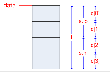
I.8.3.1. Anonymous unions
The standard of C++ makes it possible that a definition of a union only contains data members. The members of these anonymous unions appear as the variables of the environment containing the union. This environment can be a module, a function, a structure or a class.
In the following example, a and b, as well as c and f can be accessed as normal variables; however, they are stored overlapped in memory, as it is required by the union type.
static union {
    long a;
    double b;
};

int main() {
    union {
        char c[4];
        float f;
    };

    a = 2012;
    b = 1.2;    // the value of a changed!
    f = 0;
    c[0] = 1;    // the value of f changed!
}
If an anonymous union is nested within a structure (a class), its data members become the members of the structure (the class) but they will remain overlapped.
The next example illustrates how to use struct and union types together. It is often necessary that the data stored in the records of a file would have different structure for every record. Let's suppose that every record contains a name and a value, the value of which is sometimes a string sometimes a number. Memory space is spared if the two possible values are combined into a union within a structure ( variant record ):
#include <iostream>
using namespace std;

struct vrecord  {
    char type;
    char name[25];
    union {
        char address[50];
        unsigned long ID;
    };               // <---- there is no member name!
};

int main() {
    vrecord vr1={0,"BME","Budapest, Muegyetem rkpt 3-11."};
    vrecord vr2={1, "National Bank"};
    vr2.ID=3751564U;
    for (int i=0; i<2; i++) {
        cout<<"Name    : "<<vr1.name<<endl;
        switch (vr1.type) {
            case 1 :
                cout<<"ID      : "<<vr1.ID<<endl;
                break;
            case 0 :
                cout<<"Address : "<<vr1.address<<endl;
                break;
            default  :
                cout<<"Not a valid data type!"<<endl;
        }
        vr1 = vr2;
    }
}
The results:
Name : BME Address : Budapest, Muegyetem rkpt 3-11. Name : National Bank ID : 3751564 |
I.8.4. Bit fields
Classes and structures may contain members for which compilers use a space less than for integer types. Since the storage space is determined by number of bits for these members, they are called bit fields. The general declaration of bit fields:
type name_of_bitfield : bitlength;
A type can be of an integral type (enum is also). If no name is given for a bit field, an anonymous bit field is created, the function of which is to fill up the non-used bit positions. The length of a bit field has to be provided with a constant expression. The maximal value of bitlength is decided on the basis of the bit size of the biggest integer type on the given computer.
Bit fields and data members may figure in a mixed way in structure and class types:
#include <iostream>
using namespace std;

#pragma pack(1)
struct date {
   unsigned char holiday    : 1;    // 0..1
   unsigned char day        : 6;    // 0..31
   unsigned char month        : 5;    // 0..16
   unsigned short year;
};

int main() {
    date today = { 0, 2, 10, 2012 };
    date holiday = {1};
    holiday.year = 2012;
    holiday.month = 12;
    holiday .day = 25;
}
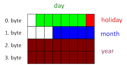
If a bit field is not given a name in its declaration, then the space of the given bit length cannot be accessed (they are used for padding). If the length of an anonymous bit field is set to 0, then the compiler forces alignment of the following data member (or bitfield) to the next int boundary.
The following example makes more comfortable the access of the line control register (LCR) of RS232 ports by using bit fields:
#include <iostream>
#include <conio.h>
using namespace std;

union LCR {
    struct {
        unsigned char datalength : 2;
        unsigned char stopbits   : 1;
        unsigned char parity     : 3;
        unsigned char            : 2;
    } bsLCR;
    unsigned char byLCR;
};

enum RS232port {eCOM1=0x3f8, eCOM2=0x2f8 };

int main() {
    LCR reg = {};
    reg.bsLCR.datalength = 3; // 8 data bits
    reg.bsLCR.stopbits = 0;   // 1 stopbit
    reg.bsLCR.parity   = 0;   // no parity
    outport(eCOM1+3, reg.byLCR);
}
The necessary operations can also be carried out with the already detailed bitwise operations; however, using bit fields make the source code more structured.
The end of the present chapter also enumerates the disadvantages of using bit fields:
The source code becomes non-portable since the position of bits within bytes or words may be different in different systems.
The address of bit fields cannot be obtained (&), since it is not sure whether they are positioned on a byte boundary.
If more variables are placed in a storage unit used together with bit fields as well, compilers generate a complementary code to manage the variables (therefore programs run slower and the size of the code increases).
Chapter II. Modular programming in C++
- II.1. The basics of functions
- II.1.1. Defining, calling and declaring functions
- II.1.2. The return value of functions
- II.1.3. Parametrizing functions
- II.1.3.1. Parameter passing methods
- II.1.3.2. Using parameters of different types
- II.1.3.2.1. Arithmetic type parameters
- II.1.3.2.2. User-defined type parameters
- II.1.3.2.3. Passing arrays to functions
- II.1.3.2.4. String arguments
- II.1.3.2.5. Functions as arguments
- II.1.3.2.6. Default arguments
- II.1.3.2.7. Variable length argument list
- II.1.3.2.8. Parameters and return value of the main() function
- II.1.4. Programming with functions
- II.2. How to use functions on a more professional level?
- II.3. Namespaces and storage classes
- II.3.1. Storage classes of variables
- II.3.2. Storage classes of functions
- II.3.3. Modular programs in C++
- II.3.4. Namespaces
- II.4. Preprocessor directives of C++
C++ supports many programming techniques. The previous part of this book focussed on structured programming , which is based on the fact that computer programs have the following three components: sequences (the statements of which are provided in the order of their execution), decisions (if, switch) and loops (while, for, do). As it can be seen, the statement goto is not included in the previous list because its usage is to be avoided.
Structured programming relies on top-down design, which consists of dividing programming tasks into smaller units until program blocks easy to handle and to test are achieved. In C and C++ languages, the smallest structural unit having independent functionality is called function .
If functions or a group of functions belonging together are put in a separate module (source file), modular programming is realised. Modules can be compiled and tested separately, and they can be imported into other projects as well. The contents of modules (compiled or source code version) can be made available for other modules by interfaces (header files in C/C++). And certain parts of these modules are hidden from the outside (data hiding). Structural programming also contributes to creating new programs from achieved modules (components) by bottom-up design.
The next parts aim at introducing our readers into modular and procedural programming in C++. Procedural programming means solving a task by subprograms (functions) that are more or less independent from one another. These subprograms call one another directly or indirectly from the main program (main()) and communicate with each other by parameters. Procedural programming can be well combined with structural and modular programming.
II.1. The basics of functions
In C++, a function is a unit (a subprogram) that has a name and that can be called from the other parts of a program as many times as it is needed. A traditional C++ program has small size and easy to handle functions. Compiled functions can be put in libraries, from which the development kit integrates the code of the referenced functions in our programs.
In order to use a function efficiently, some of its inner variables are assigned a value when the function is called. These storage units called parameters should be declared in parentheses in the function definition after the function name. When a function is called (activated), the values (arguments) to be assigned to each parameter have to be passed in a similar way.
When a function is called, arguments (if there are) are passed to the called function and control passes to the activated function. After the algorithm of a function is executed by a return statement, or the physical end of the function is reached, the called function passes control back to the place where it was called by a return statement. The value of the expression in the return statement is the return value returned back by the function, which is the result of the function call expression.
II.1.1. Defining, calling and declaring functions
C++ Standard Library provides us many useful predefined functions. We only have to declare these functions before using them. For that purpose, the corresponding header file should be included in the source code. The following table enumerates some frequently used functions and the corresponding include files:
|
function |
header file |
|---|---|
|
|
|
|
|
|
|
|
|
|
|
|
|
|
|
|
|
|
Contrary to Library functions, our own functions should always be defined as well. This function definition can be placed anywhere in a C++ program, but only once. If the definition of a function precedes the place where it is called (used), then it is also a declaration.
The general form of a function definition is the following (the signs 〈 〉 indicate optional parts): A parameter declaration list in the function header enumerates each parameter separated by each other by a comma, and every parameter is preceded by its type.
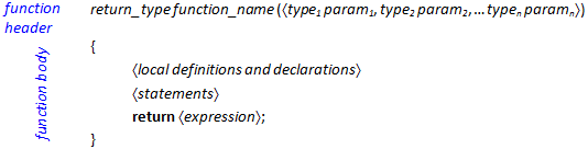
A storage class can also be given before the return type in the definition of functions. In the case of functions, the default storage class is extern, which indicates that the function can be accessed from other modules. If the accessibility of a function needs to be restricted to a given module, the static storage class should be used. (When parameters are declared, only the register storage class can be specified). If a function is intended to be placed within our own namespace, then the definition and the prototype of that function have to be put in the chosen namespace block. (Storage classes and namespaces are detailed later in this book.)
The next example contains a function that calculates the sum of the first n positive integer numbers. The function isum() expects an int type value and returns an int type result.
int isum(int n)
{
    int s = 0;
    for (int i=1; i<=n; i++)
        s += i;
    return s;
}
Suppose that in the source code, the definition of isum() is before the main () function from where the function isum() is called:
int main()
{
    cout << isum(10) << endl;
    int s = isum(7) * isum(10) + 2;
}
When a function is called , the name of the function is followed by a list of arguments separated from each other by a comma. The steps of calling a function can be traced on Figure II.2, “Steps of calling a function”.
function_name (〈argument 1 , argument 2 , … argument n 〉)
Parentheses should be used even if a function does not have any parameters. A function can be called from anywhere where a statement can be given.
The order in which arguments are evaluated is not defined by the language C++. Function call operators guarantee only one thing: by the time control is passed to a called function, the argument list has completely been evaluated (together with all of its side-effects).
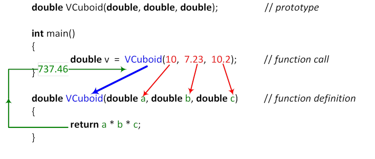
C++ standards require that functions have to be declared before they are called. Defining a function is therefore declaring a function. Then it may be logical to ask how we can make sure that the called function would always precede the place where it is called. Of course, this cannot be ensured because there are functions calling each other. In case the functions main () and isum() are swapped in the previous example, we get compilation errors until the prototype containing the whole description of the function is placed before the function is called:
int isum(int); // prototype

int main() {
 cout << isum(10) << endl;
 int s = isum(7) * isum(10) + 2;
}

int isum(int n)
{
    int s = 0;
    for (int i=1; i<=n; i++)
        s += i;
    return s;
}
The complete declaration of a function (its prototype ) contains the name and the type of the function and provides information about the number and the type of the parameters:
return_value function_name(〈parameter declaration list〉);
return_value function_name(〈type_list〉);
C++ compilers compile function calls if the prototype is already known:
checks the compatibility of the number and the types of parameters by comparing these parameters with the argument list,
converts arguments according to the types defined in the prototype and not according to the rules of automatic conversion.
(It should be noted that function definitions replace prototypes.) In most cases, a function header is used as a prototype, and it ends with a semicolon. In prototypes, parameter names do not have any importance, they can be left out or any other name can be used. The following prototypes are completely equal for compilers:
int isum(int);
int isum(int n);
int isum(int lots);
The prototype of a function can figure many times in the source code; however, they have to be the same, only parameter names can be different.
It should be noted that the prototype of functions without parameters is interpreted differently by C and C++ languages:
|
declaration |
C interpretation |
C++ interpretation |
|---|---|---|
|
type funct(); |
type funct(...); |
type funct(void); |
|
type funct(...); |
type funct(...); |
type funct(...); |
|
type funct(void); |
type funct(void); |
type funct(void); |
C++ makes it possible that a parameter list containing at least one parameter should end with three dots (...). A function defined in that way can be called with at least one parameter but also with any number or type of arguments. Let's look at the prototype of the function sscanf ().
int sscanf ( const char * str, const char * format, ...);
Chapter (Section I.5, “Exception handling”) dealing with exceptions also mentioned that the transferring (throw) of exceptions to the caller function can be enabled or disabled in function header. When the keyword throw is used, the definition of functions is modified in the following way:
return_type function_name (〈parameterlist〉) 〈throw(〈type_list〉)〉
{
〈local definitions and declarations〉
〈statements〉
return 〈expression〉;
}
The prototype corresponding to the definition also has to contain the keyword throw:
return_type function _ name (〈parameterlist〉) 〈throw(〈type_list〉)〉;
Let's see some prototypes mentioning the type of the thrown exceptions:
int funct() throw(int, const char*); // int and const char*
int funct();                   // all
int funct() throw();               // not any
II.1.2. The return value of functions
The return_type figuring in the definition/declaration of a function determines the return type of the function, which can be of any C++ type with the exception of arrays and functions. Functions cannot return data with volatile or const type qualifiers; however, they can return a reference or a pointer to such data.
When the return statement is processed, the function passes control back to the caller, and the return value of type return_type can be used in the place where the function has been called.
return expression;
Within a function, many return statements may be placed; however, structured programming requires that if it is possible, only one exit point should be used.
The following prime number checker function can be exited at three points because there are three return statements, which results in a program structure more difficult to understand globally.
bool IsPrime(unsigned n)
{
    if (n<2) // 0, 1
        return false;
    else {
        unsigned limit = (unsigned)sqrt(1.0*n);
        for (unsigned d=2; d<=limit; d++)
            if ((n % d) == 0)
                return false;
    }
    return true;
}
If an additional variable (result) is introduced, the code becomes much clearer:
bool IsPrime(unsigned n)
{
    bool result = true;
    if (n<2) // 0, 1
        result = false;
    else {
        unsigned limit = (unsigned)sqrt(1.0*n);
        for (unsigned d=2; d<=limit && result; d++)
            if ((n % d) == 0)
                result = false;
    }
    return result;
}
By using the type void, we can create functions that do not return any value. (Other programming languages call these procedures.) In that case, exiting the function is carried out by a return statement without a return value. Functions of type void are mostly exited when the closing curly bracket is reached.
The following function prints out all perfect numbers within a given interval. (A positive integer number is perfect if the sum of its positive divisors is equal to the given number. The smallest perfect number is 6 because 6 = 1+2+3, but 28 is also perfect because 28 = 1+2+4+7+14.)
void PerfectNumbers(int from, int to)
{
      int sum = 0;
      for(int i=from; i<=to; i++) {
          sum = 0;
          for(int j=1; j<i; j++) {
              if(i%j == 0)
                  sum += j;
          }
          if(sum == i)
              cout<< i <<endl;
      }
 }
Functions can return pointers or references; however, it is forbidden to return local variables or the address of local variables since they are deleted when the function is exited. Let's see some good solutions.
#include <cassert>
#include <new>
using namespace std;

double * Allocate(int size) {
    double *p = new (nothrow) double[size];
    assert(p);
    return p;
}

int  & DinInt() {
    int *p = new (nothrow) int;
    assert(p);
    return *p;
}

int main() {
    double *pd = Allocate(2012);
    pd[2] = 8;
    delete []pd;

    int &x = DinInt();
    x = 10;
    delete &x;
}
The function named Allocate() allocates an array of type double with a given number of elements and returns the beginning address of the dynamic array. The function DinInt() allocates space on the heap for only one integer variable and returns the reference of the dynamic variable. This value can be accessed by a variable of reference type, the dynamic variable can be accessed without the * operator.
II.1.3. Parametrizing functions
When we create functions we have to tend to use the algorithm in the function in a range as wide as possible. This is needed because the input values (parameters) of an algorithm are assigned when the function is called. The following function without a parameter prints out a greeting:
void Greeting(void) {
cout << "Welcome on board!" << endl;
}
Every time this function is called, we always get the same message:
Greeting();
What should we do to greet users according to the part of the day? Then, the function should be parametrized:
#include <iostream>
#include <string>
using namespace std;
void Greeting(string greeting) {
cout << greeting << endl;
}
int main() {
Greeting("Good morning");
Greeting("Good evening!");
}
In a C++ function definition, each parameter is preceded by its type, no simplification is allowed. A declared parameter can be used as a local variable within a function; however, it is only accessible from the outside when they are passed as arguments. A parameter can be scalar (bool, char, wchar_t, short, int, long, long long, float, double, enumeration, reference and pointer) or structure, union, class or array.
In order to demonstrate these different types of parameters, let's make the function calculating the value of a polynomial on the basis of Horner's method.
The general form of polynomials: 
Horner's scheme 
The input parameters of the function are: the value of x, the degree of the polynomial and an array of the coefficients of the polynomial (having degree+1 elements). (The type qualifier const forbids the modification of the elements of the array within the function.)
double Polynomial(double x, int n, const double c[]) {
double y = 0;
for (int i = n; i > 0; i--)
y = (y + c[i]) * x;
return y + c[0];
}
int main(){
const int degree = 3;
double coefficients[degree + 1] = { 5, 2, 3, 1};
cout << Polynomial(2,degree,coefficients)<< endl; // 29
}
II.1.3.1. Parameter passing methods
In the language C++ parameters can be grouped in two categories on the basis of how they are passed. There are input parameters passed by value and variable parameters passed by reference.
II.1.3.1.1. Passing parameters by value
If parameters are passed by value , it is their value that is passed to the called function. The parameters of the function are initialised to the passed values, and after, the relation between these arguments and parameters ends. As a consequence, the operations carried out on parameters have no effect on the arguments with which the function is called.
Arguments can only be expressions, the type of which can be converted into the type of the corresponding parameters of the called function.
The function enumber() returns the approximate value of e by summing up the first n+1 elements of the sequence:

double enumber(int n) {
double f = 1;
double eseq = 1;
for (int i=2; i<=n; i++) {
eseq += 1.0 / f;
f *= i;
}
return eseq;
}
The function enumber() can be called by any numeric expression:
int main(){
long x =1000;
cout << enumber(x)<< endl;
cout << enumber(123) << endl;
cout << enumber(x + 12.34) << endl;
cout << enumber(&x) << endl;
}
When it is first called, the value of the variable x of type long is passed to the function converted to type int. In the second case, the value of the parameter becomes a constant of type int. The argument of the third call is an expression of type double, the value of which is converted to an integer before it is passed. This conversion may provoke data loss - that is why the compiler sends us an alert message. The last case is an odd-one-out in the list of the calls since in that case, the compiler rejects to convert the address of the variable x to an integer. Since type conversions of this type can lead to run-time errors, conversions have to be asked for separately:
cout << enumber((int)&x) << endl;
If the value of an external variable is intended to be modified within the function, it is the address of the variable that have to be passed and the address has to be received as a parameter of pointer type. As an example, let's have a look at the classical function swapping the values of two variables:
void pswap(double *p, double *q) {
double c = *p;
*p = *q;
*q = c;
}
int main(){
double a = 12, b =23;
pswap(&a, &b);
cout << a << ", " << b<< endl; // 23, 12
}
Arguments may also be expressions, but in that case these expressions have to be left value expressions. It should be noted that arrays are passed to functions by their beginning address.
If the type qualifier const is placed in the parameter list, we can restrict the modification of the memory space to which a pointer points ( const double *p) and restrict the modification of the value of the pointer ( double * const p) within a function.
II.1.3.1.2. Passing parameters by reference
Parameters passed by value are used as local variables in functions. However, reference parameters are not independent variables; they are only alternative names for the arguments provided in a function call.
Reference parameters are marked with a & character placed between the type and the parameter name in the function header. When the function is called, the argument variables have to have the same type as that of parameters. The function swapping the value of variables becomes simpler if we use parameters passed by reference:
void rswap(double & a, double & b) {
double c = a;
a = b;
b = c;
}
int main(){
double x = 12, y =23;
rswap(x, y);
cout << x << ", " << y << endl; // 23, 12
}
The value (right-value) and the address (left-value) of a reference parameter equals with the value and the address of the referenced variable, so it completely replaces the latter.
It should be noted that the compiled code of the functions pswap() and rswap() are completely the same in Visual Studio. That is why it is not more efficient to use pswap() in C++ program codes.
Independently of the parameter passing method, compilers allocate memory space for parameters in the stack. In the case of value parameters, the size of the allocated memory depends on the type of the parameter; therefore it can be really big, while in the case of reference parameters it is the pointer size used in the given system that counts. In the case of a bigger structure or object, we should not only consider the increased memory need but also the longer time a function call requires.
In the following example, a reference to a structure is passed to a function but we would like to prevent the modification of the structure within the function. For that purpose, the most efficient method is to use a parameter of constant reference type :
#include <iostream>
#include <cstdlib>
#include <ctime>
using namespace std;
struct svector {
int size;
int a[1000];
};
void MinMax(const svector & sv, int & mi, int & ma) {
mi = ma = sv.a[0];
for (int i=1; i<sv.size; i++) {
if (sv.a[i]>ma)
ma = sv.a[i];
if (sv.a[i]<mi)
mi = sv.a[i];
}
}
int main() {
const int maxn = 1000;
srand(unsigned(time(0)));
svector v;
v.size=maxn;
for (int i=0; i<maxn; i++) {
v.a[i]=rand() % 102 + (rand() % 2012);
}
int min, max;
MinMax(v, min, max);
cout << min << endl;
cout << max << endl;
}
It should be noted that while in the solution above calling the function MinMax() is faster and less memory space is required in the stack, however accessing parameters within the function is more efficient by using value type parameters.
Constant reference parameters completely replace constant value parameters, so any expression (not only variables) can be used as arguments. This fact is demonstrated by the example determining the greatest common divisor of two numbers:
int Gcd(const int & a, const int & b ) {
int min = a<b ? a : b, gcd = 0;
for (int n=min; n>0; n--)
if ( (a % n == 0) && (b % n) == 0) {
gcd = n;
break;
}
return gcd;
}
int main() {
cout << Gcd(24, 32) <<endl; // 8
}
II.1.3.2. Using parameters of different types
The following subchapters will broaden our knowledge about parameters for different types with the help of examples. In the examples of this subchapter, the definition of functions is followed by the presentation of the function call after a dotted line. Of course, we give the whole program code for more complicated cases.
II.1.3.2.1. Arithmetic type parameters
Parameters can be declared by the types bool, char, wchar_t, int, enum, float and double and these types can also be function types.
In general, we do not have to hesitate much when deciding what the used parameters and the returned value will be. If a function does not return any value, i.e. it only carries out an operation, then we use the return type void and value parameters:
void PrintOutF(double data, int field, int precision) {
cout.width(field);
cout.precision(precision);
cout << fixed << data << endl;
}
...
PrintOutF(123.456789, 10, 4); // 123.4568
We also have an easy task when a function returns one value from the input values:
long Product(int a, int b) {
return long(a) * b;
}
...
cout << Product(12, 23) <<endl; // 276
However, if we want a function to return more values, then the solution should be based on reference (or pointer) parameters. In that case, the function is of type void or of a type that indicates the successfulness of an operation, for example bool. The following function Cube() calculates the surface area, the volume and the length of the body diagonal of the cube on the basis of its edge length:
void Cube(double a, double & surface_area, double & volume,
double & diagonal) {
surface_area = 6 * a * a;
volume = a * a * a;
diagonal = a * sqrt(3.0);
}
...
double f, v, d;
Cube(10, f, v, d);
II.1.3.2.2. User-defined type parameters
If user-defined types (struct, class, union) are used in parameter lists or a return value, then the solutions presented for arithmetic types can be used. The basis of that is provided by the fact that C++ defines value assignment between objects and unions of the same type.
Arguments of user-defined types can be passed to functions by value, by reference or by a pointer. In the standard C++, the return value of functions can be of a user-defined type. Therefore there are many possibilities. We only have to decide which one is the best for the given task.
As an example, let's see a structure appropriate for storing complex numbers.
struct complex {
double re, im;
};
Let's create a function to add two complex numbers. Its members and the structure that stores the result are passed to the function with a pointer to them (CSum1()). Since input parameters are not intended to be modified within the function, the type qualifier const is used.
void CSum1(const complex*pa, const complex*pb, complex *pc){
pc->re = pa->re + pb->re;
pc->im = pa->im + pb->im;
}
The second function returns the sum of the two complex numbers passed by value (CSum2()). Addition is carried out in a local structure, and it is only its value that is passed by the return statement.
complex CSum2(complex a, complex b) {
complex c;
c.re = a.re + b.re;
c.im = a.im + b.im;
return c;
}
The second solution is of course much safer and expresses more the essential of this operation than the first one. In any other aspect (memory need, speed), we have to choose the first function. However, if a reference type is used, the solution we get realises the advantages of the function CSum2() and is also able to beat the function CSum1().
complex Csum3(const complex & a, const complex & b) {
complex c;
c.re = a.re + b.re;
c.im = a.im + b.im;
return c;
}
The three different solutions require two different function calls. The following main() function contains a call for all the three adding function:
int main() {
complex c1 = {10, 2}, c2 = {7, 12}, c3;
// all the three arguments are pointers
CSum1(&c1, &c2, &c3);
c3 = CSum2(c1, c2); // arguments are structures
// arguments are structure references
c3 = CSum3(c1, c2);
}
II.1.3.2.3. Passing arrays to functions
Now let's see how we can pass arrays to functions in C++. We have already mentioned that arrays cannot be passed or returned by value (by copying their values). There is even a difference between passing one-dimensional arrays (vectors) and multi-dimensional ones as arguments.
If one-dimensional arrays (vectors) are passed as function arguments, it is a pointer to their first value that is passed. That is why, the modifications carried out on the elements of the vector within the function will remain even after the function is exited.
Parameters of a vector type can be declared either as pointers or with empty indexing operators . Since C++ arrays do not contain any information about the number of their elements, the latter information should also be passed as a separate parameter. Within functions, accessing their elements can be done by any of the already presented two methods (indexing, pointer). A function calculating the sum of the first n elements of a vector of type int can be realised in many ways. The parameters of the vector should be qualified as const because that ensures that the vector elements could not be modified within the function.
long VectorSum1 (const int vector[], int n) {
long sum = 0;
for (int i = 0; i < n; i++) {
sum+=vector[i]; // or sum+=*(vector+i);
}
return sum;
}
...
int v[7] = { 10, 2, 11, 30, 12, 7, 23};
cout <<VectorSum1(v, 7)<< endl; // 95
cout <<VectorSum1(v, 3)<< endl; // 23
However, there is a solution that is completely equal to the solution above: if the address of the vector is received in a pointer. (The second const qualifier makes it impossible to modify the pointer value.)
long VectorSum2 (const int * const vector, int n) {
long sum = 0;
for (int i = 0; i < n; i++) {
sum+=vector[i]; // or sum+=*(vector+i);
}
return sum;
}
In case the elements of a passed vector have to be modified, for example, they have to be sorted, the first const type qualifier has to be left out:
void Sort(double v[], int n) {
double temp;
for (int i = 0; i < n-1; i++)
for (int j=i+1; j<n; j++)
if (v[i]>v[j]) {
temp = v[i];
v[i] = v[j];
v[j] = temp;
}
}
int main() {
const int size=7;
double v[size]={10.2, 2.10, 11, 30, 12.23, 7.29, 23.};
Sort(v, size);
for (int i = 0; i < size; i++)
cout << v[i]<< '\t';
cout << endl;
}
One-dimensional arrays can be passed by reference , too. However, in that case, the size of the vector to be processed has to be fixed.
long VectorSum3 (const int (&vector)[6]) {
long sum = 0;
for (int i = 0; i < 6; i++) {
sum+=vector[i]; // or sum+=*(vector+i);
}
return sum;
}
...
int v[6] = { 10, 2, 11, 30, 12, 7};
cout << VectorSum3(v) << endl;
When two-dimensional array arguments are presented, we mean by the notion of two-dimensional arrays the arrays that are created (in a static way) by the compiler:
int m[2][3];
A reference to the elements of the array (m[i][j]) can also be expressed in the form *(( int *)m+(i*3)+j) (in fact, that is what compilers also do). From that expression, it can be clearly seen that the second dimension of two-dimensional arrays (3) has a vital importance for compilers, while the number of rows can be anything.
Our aim is to make a function that prints out the elements of a two-dimensional integer array of any size in a matrix form. As a first step, let's create the version of this function that is able to print out arrays of size 2x3.
void PrintMatrix23(const int matrix[2][3]) {
for (int i=0; i<2; i++) {
for (int j=0; j<3; j++)
cout <<matrix[i][j] <<'\t';
cout<<endl;
}
}
...
int m[2][3] = { {10, 2, 12}, {23, 7, 29} };
PrintMatrix23(m);
10 2 12 23 7 29 |
The two-dimensional array is passed to the function as a pointer to the start of the used memory space. When accessing array elements, the compiler makes use of the fact that rows contain 3 elements. In that way, the function above can simply be transformed into another function that prints out an array of any nx3 size, we only have to pass the number of rows as a second argument:
void PrintMatrixN3(const int matrix[][3], int n) {
for (int i=0; i<n; i++) {
for (int j=0; j<3; j++)
cout <<matrix[i][j] <<'\t';
cout<<endl;
}
}
...
int m[2][3] = { {10, 2, 12}, {23, 7, 29} };
PrintMatrixN3(m, 2);
cout << endl;
int m2[3][3] = { {1}, {0, 1}, {0, 0, 1} };
PrintMatrixN3(m2, 3);
10 2 12 23 7 29 1 0 0 0 1 0 0 0 1 |
However, there is no possibility to leave out the second dimension because in that case the compiler is not able to identify the rows of the array. We can only do one thing to get a general solution: we take over the task of accessing the memory space of the array from the compiler by using the above mentioned expression:
void PrintMatrixNM(const void *pm, int n, int m) {
for (int i=0; i<n; i++) {
for (int j=0; j<m; j++)
cout <<*((int *)pm+i*m+j) <<'\t';
cout<<endl;
}
}
...
int m[2][3] = { {10, 2, 12}, {23, 7, 29} };
PrintMatrixNM(m, 2, 3);
cout << endl;
int m2[4][4] = { {0,0,0,1}, {0,0,1}, {0,1}, {1} };
PrintMatrixNM(m2, 4, 4);
10 2 12 23 7 29 0 0 0 1 0 0 1 0 0 1 0 0 1 0 0 0 |
II.1.3.2.4. String arguments
When creating functions, we can also choose between C-style (char vector) or user-defined type ( string ) string processing. Since we have already presented both parameter types, we only show here some examples.
Processing character sequences can be done in three ways. First, strings are treated as vectors (with the help of indexes), or we can carry out the necessary operations by pointers or finally we can use the member functions of the type string .
It should be noted that modifying the content of string literals (character sequence constants) leads in general to a run-time error, therefore they can only be passed to functions as constants or a value parameter of type string .
In the first example, we only iterate through the elements of a character sequence while counting the number of occurrence of a given character.
If a string is processed as a vector , we need an index variable (i) to index its characters. The condition that stops counting is fulfilled if the 0 byte closing the character sequence is reached. In the meanwhile, the index variable is incremented continuously by one.
unsigned CountChC1(const char s[], char ch) {
unsigned cnt = 0;
for (int i=0; s[i]; i++) {
if (s[i] == ch)
cnt++;
}
return cnt;
}
If we use a pointer , we go through all characters by incrementing the pointer pointing first to the beginning of the character sequence until we reach the final '\0' character (byte 0).
unsigned CountChC2(const char *s, char ch) {
unsigned cnt = 0;
while (*s) {
if (*s++ == ch)
cnt++;
}
return cnt;
}
If the string has the type string , its member functions can also be used besides indexing:
unsigned CountChCpp(const string & s, char ch) {
int cnt = -1, position = -1;
do {
cnt++;
position = s.find(ch, position+1);
} while (position != string::npos);
return cnt;
}
The corresponding function calls are demonstrated with a string constant, a character array and a string type argument. All the three functions can be called with a string literal or a character array argument:
char s1[] = "C, C++, Java, C++/CLI / C#";
string s2 = s1;
cout<<CountChC1("C, C++, Java, C++/CLI / C#", 'C')<<endl;
cout<<CountChC2(s1, 'C')<<endl;
However, if we use arguments of type string , the first two functions need a little manipulation:
cout << CountChC2(s2.c_str(), 'C') << endl; cout << CountChCpp(s2, 'C') << endl;
Conditions become more strict if the declaration const is left out before the parameters. The next example reverses the string passed to the function, and returns a pointer to the new string. The solution is carried out on all the three cases presented above:
char * StrReverseC1(char s[]) {
char ch;
int length = -1;
while(s[++length]); // determining the string length
for (int i = 0; i < length / 2; i++) {
ch = s[i];
s[i] = s[length-i-1];
s[length-i-1] = ch;
}
return s;
}
char * StrReverseC2(char *s) {
char *q, *p, ch;
p = q = s;
while (*q) q++; // going through the elements until byte 0 closing the string
p--; // p points to the first character of the string
while (++p <= --q) {
ch = *p;
*p = *q;
*q = ch;
}
return s;
}
string& StrReverseCpp(string &s) {
char ch;
int length = s.size();
for (int i = 0; i < length / 2; i++) {
ch = s[i];
s[i] = s[length-i-1];
s[length-i-1] = ch;
}
return s;
}
The functions have to be called by arguments having the same type as the parameters:
int main() {
char s1[] = "C++ programming";
cout << StrReverseC1(s1) << endl; // gnimmargorp ++C
cout << StrReverseC2(s1) << endl; // C++ programming
string s2 = s1;
cout << StrReverseCpp(s2) << endl; // gnimmargorp ++C
cout << StrReverseCpp(string(s1)); // gnimmargorp ++C
}
II.1.3.2.5. Functions as arguments
When developing mathematical applications, it is normal to expect that a well elaborated algorithm could be used in many functions. For that purpose, the function has to be passed as an argument to the function executing the algorithm.
II.1.3.2.5.1. Function types and typedef
With typedef, the type of a function can be indicated by a synonymous name. The function type declares the function that has the given number and type of parameters and returns the given data type. Let's have a look at the following example function that calculates the value of the third degree polynomial  if x is given. The prototype and the definition of the function are:
double poly3(double); // prototype
double poly3(double x) // definition
{
return x*x*x - 6*x*x - x + 30;
}
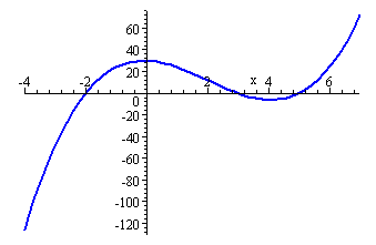
Let's have a look at the prototype of the function and let's type typedef before it and replace the name poly3 with mathfunction.
typedef double mathfunction(double);
If the type mathfunction is used, the prototype of the function poly3() is:
mathfunction poly3;
II.1.3.2.5.2. Pointers to functions
In C++, function names can be used in two ways. A function name can be the left operand of a function call operator: in this case, it is a function call expression
poly3(12.3)
the value of which is the value returned by the function. However, if the function name is used alone
poly3
we get a pointer, the value of which is a memory address where the code of the function is (code pointer) and the type of which is that of the function.
Let's define a pointer to the function poly3(). This pointer can be assigned the address of the function poly3() as a value. The definition can be obtained easily if the name in the header of the function poly3 is replaced by the expression (*functionptr):
double (*functionptr)(double);
functionptr is a pointer to a function that returns a double value and that has a parameter of type double.
However, this definition can be provided in a much more legible way if we use the type mathfunction created with typedef:
mathfunction *functionptr;
When the pointer functionptr is initialised, the function poly3 can be called indirectly:
functionptr = poly3;
double y = (*functionptr)(12.3);
or
double y = functionptr(12.3);
If we want to create a reference to this function, we have to follow the same steps. But in this case, the initial value has to be given already in the definition:
double (&functionref)(double) = poly3;
or
mathfunction &functionref = poly3;
Calling the function by using the reference:
double y = functionref(12.3);
II.1.3.2.5.3. Examples for pointers to functions
On the basis of the things said above, the prototype of the Library function qsort () becomes more comprehensible:
void qsort(void *base, size_t n, size_t width,
int (*fcmp)(const void *, const void *));
With qsort (), we can sort data stored in an array by using the Quicksort algorithm. This function makes it possible to sort an array starting at the address base, having n number of elements and each element being allocated width bytes. The comparator function called during sorting has to be provided by ourselves as the parameter fcmp.
The following example uses the function qsort () to sort integer and string arrays:
#include <iostream>
#include <cstdlib>
#include <cstring>
using namespace std;
int icmp(const void *p, const void *q) {
return *(int *)p-*(int *)q;
}
int scmp(const void *p, const void *q) {
return strcmp((char *)p,(char *)q);
}
int main() {
int m[8]={2, 10, 7, 12, 23, 29, 11, 30};
char names[6][20]={"Dennis Ritchie", "Bjarne Stroustrup",
"Anders Hejlsberg","Patrick Naughton",
"James Gosling", "Mike Sheridan"};
qsort(m, 8, sizeof(int), icmp);
for (int i=0; i<8; i++)
cout<<m[i]<<endl;
qsort(names, 6, 20, scmp);
for (int i=0; i<6; i++)
cout<<names[i]<<endl;
}
The function named tabulate() in the following example codes can be used to print out in tabular form the values of any function having a parameter of type double and returning a double value. The parameters of the function tabulate() contains the two interval boundaries and the step value.
#include <iostream>
#include <iomanip>
#include <cmath>
using namespace std;
// Prototypes
void tabulate(double (*)(double), double, double, double);
double sqr(double);
int main() {
cout<<"\n\nThe values of the function sqr() ([-2,2] dx=0.5)"<<endl;
tabulate(sqr, -2, 2, 0.5);
cout<<"\n\nThe values of the function sqrt() ([0,2] dx=0.2)"<<endl;
tabulate(sqrt, 0, 2, 0.2);
}
// The definition of the function tabulate()
void tabulate(double (*fp)(double), double a, double b,
double step){
for (double x=a; x<=b; x+=step) {
cout.precision(4);
cout<<setw(12)<<fixed<<x<< '\t';
cout.precision(7);
cout<<setw(12)<<fixed<<(*fp)(x)<< endl;
}
}
// The definition of the function sqr()
double sqr(double x) {
return x * x;
}
The results:
The values of the function sqr() ([-2,2] dx=0.5)
-2.0000 4.0000000
-1.5000 2.2500000
-1.0000 1.0000000
-0.5000 0.2500000
0.0000 0.0000000
0.5000 0.2500000
1.0000 1.0000000
1.5000 2.2500000
2.0000 4.0000000
The values of the function sqrt() ([0,2] dx=0.2)
0.0000 0.0000000
0.2000 0.4472136
0.4000 0.6324555
0.6000 0.7745967
0.8000 0.8944272
1.0000 1.0000000
1.2000 1.0954451
1.4000 1.1832160
1.6000 1.2649111
1.8000 1.3416408
2.0000 1.4142136
|
II.1.3.2.6. Default arguments
In the prototype of C++ functions, certain parameters can be assigned a so-called default value. Compilers use these values if there is no argument corresponding to the given parameter when the function is called:
// prototype
long SeqSum(int n = 10, int d = 1, int a0 = 1);
long SeqSum(int n, int d, int a0) { // definition
long sum = 0, ai;
for(int i = 0; i < n; i++) {
ai = a0 + d * i;
cout << setw(5) << ai;
sum += ai;
}
return sum;
}
The function named SeqSum() creates an arithmetic sequence of n elements. The first element is a0, the difference between elements is d. The function returns the sum of the elements of the sequence.
It should be noted that parameters having a default value are placed one after another continuously from right to left, while arguments have to be provided continuously from left to right when the function is called. If a prototype is used, default values can only be provided in the prototype.
Now let's have a look at the value of the parameters after some possible calls of the function above.
|
Call |
Parameters | ||
|---|---|---|---|
|
n |
d |
a0 | |
|
SeqSum() |
10 |
1 |
1 |
|
SeqSum(12) |
12 |
1 |
1 |
|
SeqSum(12,3) |
12 |
3 |
1 |
|
SeqSum(12, 3, 7) |
12 |
3 |
7' |
Default arguments make functions more flexible. For example, if a function is often called with the same argument list, it is worth making frequently used parameters default and calling the function without those arguments.
II.1.3.2.7. Variable length argument list
There are cases when the number and the type of the parameters of a function are not known in advance. In the declaration of these functions, the parameter list ends with an ellipsis (three dots):
int printf(const char * format, ... );
The ellipsis indicates to the compiler that further arguments can be expected. The function printf () (cstdio) has to be called by at least one argument but this can be followed by other arguments the number of which is not specified:
char name[] = "Bjarne Stroustrup";
double a=12.3, b=23.4, c=a+b;
printf("C++ language\n");
printf("Name: %s \n", name);
printf("Result: %5.3f + %5.3f = %8.4f\n", a, b, c);
The function printf () processes the next argument on the basis of format.
When functions with similar declaration are called, compilers only check the type of the parameters and that of the arguments until they reach the "..." element. After that, passing the arguments to the function is carried out on the basis of the type of the given (or eventually converted) arguments.
C++ makes it possible to use the ellipsis in our own functions, i.e. variable length argument lists. In order that the value of the passed arguments be found in the memory space containing the parameters, the first parameter always has to be provided.
C++ standard contains some macros with the help of which a variable length argument list can be processed. The macros defined in the header file cstdarg use pointers of type va_list to access arguments:
|
|
returns the following element in the argument list. |
|
|
cleaning up after all arguments are processed. |
|
|
initializes the pointer used to access the arguments. |
As an example, let's look at the function Average(), which calculates the average of any number of values of type double. The number of the elements has to be provided as the first argument.
#include<iostream>
#include<cstdarg>
using namespace std;
double Average(int num, ... ) {
va_list numbers;
// passing through the first (num) arguments
va_start(numbers, num);
double sum = 0;
for(int i = 0; i < num; ++i ) {
// accessing the double arguments
sum += va_arg(numbers, double);
}
va_end(numbers);
return (sum/num);
}
int main() {
double avg = Average(7,1.2,2.3,3.4,4.5,5.6,6.7,7.8);
cout << avg << endl;
}
II.1.3.2.8. Parameters and return value of the main() function
The interesting thing about the main () function is not only that program execution starts here but also that it can have many parameterizing options:
int main( ) int main( int argc) ( ) int main( int argc, char *argv[]) ( )
argv points to an array (a vector) of character pointers, argc gives the number of strings in the array. (The value of argc is at least 1 since argv[0] refers to the character sequence containing the name of the program.)
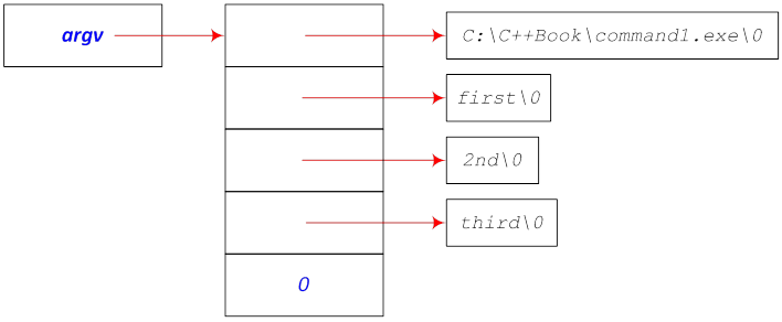
The return value of main (), which is of an int type according to the standard, can be provided within the main () function in a return statement or as an argument of the Standard Library function exit () that can be placed anywhere in a program. The header file cstdlib contains standard constants:
#define EXIT_SUCCESS 0 #define EXIT_FAILURE 1
These can be used as an exit code signalling whether the execution of the program was successful or not.
The main () function differs from other normal C++ functions in many ways: it cannot be declared as a static or inline function, it is not obligatory to use return in it and it cannot be overloaded. On the basis of the recommendations of C++ standards, it cannot be called within a program and its address cannot be obtained.
The following command1.cpp program prints out the number of arguments and then all of its arguments:
#include <iostream>
using namespace std;
int main(int argc, char *argv[]) {
cout << "number of arguments: " << argc << endl;
for (int narg=0; narg < argc; narg++)
cout << narg << " " << argv[narg] << endl;
return 0;
}
Command line arguments can be provided in the console window
C:\C++Book>command1 first 2nd third
or in the Visual Studio development environment (Figure II.5, “Providing command line arguments”).
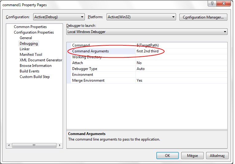
The results of executing command1.exe:
|
In a console window |
In a development environment |
|---|---|
C:\C++Book>command1 first 2nd third number of arguments: 4 0 command1 1 first 2 2nd 3 third C:\C++Book> |
C:\C++Book>command1 first 2nd third number of arguments: 4 0 C:\C++Book\command1.exe 1 first 2 2nd 3 third C:\C++Book> |
The next example code (command2.cpp) demonstrates a solution easy to use when creating utility software to test whether input arguments are well provided or not. The program only starts if it is called with two arguments. Otherwise, it sends an error message and prints out how to start the program from the command line properly.
#include <iostream>
#include <cstdlib>
using namespace std;
int main(int argc, char *argv[]) {
if (argc !=3 ) {
cerr<<"Wrong number of parameters!"<<endl;
cerr<<"Usage: command2 arg1 arg2"<<endl;
return EXIT_FAILURE;
}
cout<<"Correct number of parameters:"<<endl;
cout<<"1. argument: "<<argv[1]<<endl;
cout<<"2. argument: "<<argv[2]<<endl;
return EXIT_SUCCESS;
}
The results of the execution of command2.exe:
|
Wrong number of parameters: command2 |
Correct number of parameters: command2 alfa beta |
|---|---|
Wrong number of parameters! Usage: command2 arg1 arg2 |
Correct number of parameters: 1. argument: alfa 2. argument: beta |
II.1.4. Programming with functions
Procedural programming requires that separate functions be created for each subtask and that these functions could be tested separately. Solving the original task is achieved by calling these already tested functions. It is important to arrange communication between these functions. As we have already seen in some functions, parameterizing and return values represent this communication. However, in the case of functions being in a logical relationship with one another, there are more possibilities that can even increase the efficiency of the solution.
As an example, let's have a look at a task everybody knows: determining the area and the perimeter of a triangle. Calculating the area is carried out with Heron's formula , the prerequisite of which is the fulfilment of triangle inequality. This states that every side of a triangle is smaller that the sum of the two other sides.
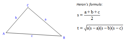
The solution consisting of only the main () function can be realised easily even if we have read only the first some chapters of this book:
#include <iostream>
#include <cmath>
using namespace std;
int main() {
double a, b, c;
do {
cout <<"a side: "; cin>>a;
cout <<"b side: "; cin>>b;
cout <<"c side: "; cin>>c;
} while(!((a<b+c) && (b<a+c) && (c<a+b)));
double p = a + b + c;
double s = p/2;
double area = sqrt(s*(s-a)*(s-b)*(s-c));
cout << "perimeter: " << p <<endl;
cout << "area: " << area <<endl;
}
This program is very simple but it has some drawbacks because it cannot be reused and its structure is not easy to understand.
II.1.4.1. Exchanging data between functions using global variables
The solution of the problem above can be divided into parts that are logically independent of each other, more precisely:
reading the three side lengths of the triangle,
checking Triangle inequality,
calculating the perimeter,
calculating the area
and printing out calculated data.
The first four of the above mentioned activities will be realized by independent functions that communicate with each other and the main() function by shared (global) variables. Global variables should be provided outside function blocks and before the functions. (We should not forget about providing the prototypes!)
#include <iostream>
#include <cmath>
using namespace std;
// global variables
double a, b, c;
// prototypes
void ReadData();
bool TriangleInequality();
double Perimeter();
double Area();
int main() {
ReadData();
cout << "perimeter: " << Perimeter()<<endl;
cout << "area: " << Area()<<endl;
}
void ReadData() {
do {
cout <<"a side: "; cin>>a;
cout <<"b side: "; cin>>b;
cout <<"c side: "; cin>>c;
} while(!TriangleInequality() );
}
bool TriangleInequality() {
if ((a<b+c) && (b<a+c) && (c<a+b))
return true;
else
return false;
}
double Perimeter() {
return a + b + c;
}
double Area() {
double s = Perimeter()/2;
return sqrt(s*(s-a)*(s-b)*(s-c));
}
It's clear that the code has become more legible; however, it still cannot benefit from a broader use. For example, if we want to store the data of other triangles as well and to reuse them later in other tasks, we have to make sure to set appropriately the global variables a, b and c.
int main() {
double a1, b1, c1, a2, b2, c2;
ReadData();
a1 = a, b1 = b, c1 = c;
ReadData();
a2 = a, b2 = b, c2 = c;
a = a1, b = b1, c = c1;
cout << "perimeter: " << Perimeter()<<endl;
cout << "area: " << Area()<<endl;
a = a2, b = b2, c = c2;
cout << "perimeter: " << Perimeter()<<endl;
cout << "area: " << Area()<<endl;
}
Therefore, the solution would be better if the data of triangles are passed to the concerned functions as arguments.
II.1.4.2. Exchanging data between functions using parameters
Now we will not detail the following solutions since we have already presented the things to know about that in the previous sections.
#include <iostream>
#include <cmath>
using namespace std;
void ReadData(double &a, double &b, double &c);
bool TriangleInequality(double a, double b, double c);
double Perimeter(double a, double b, double c);
double Area(double a, double b, double c);
int main() {
double x, y, z;
ReadData(x , y , z);
cout << "perimeter: " << Perimeter(x, y, z)<<endl;
cout << "area: " << Area(x, y, z) <<endl;
}
void ReadData(double &a, double &b, double &c) {
do {
cout <<"a side: "; cin>>a;
cout <<"b side: "; cin>>b;
cout <<"c side: "; cin>>c;
} while(!TriangleInequality(a, b, c) );
}
bool TriangleInequality(double a, double b, double c) {
if ((a<b+c) && (b<a+c) && (c<a+b))
return true;
else
return false;
}
double Perimeter(double a, double b, double c) {
return a + b + c;
}
double Area(double a, double b, double c) {
double s = Perimeter(a, b, c)/2;
return sqrt(s*(s-a)*(s-b)*(s-c));
}
Now let's see the main () function if two triangles are to be dealt with.
int main() {
double a1, b1, c1, a2, b2, c2;
ReadData(a1, b1, c1);
ReadData(a2, b2, c2);
cout << "perimeter: " << Perimeter(a1, b1, c1)<<endl;
cout << "area: " << Area(a1, b1, c1)<<endl;
cout << "perimeter: " << Perimeter(a2, b2, c2)<<endl;
cout << "area: " << Area(a2, b2, c2)<<endl;
}
When the two methods are compared with respect to speed, we could observe that global variables make programs run faster (and therefore they become more efficient) since arguments are not copied to the stack before a function is called. We have also seen the drawbacks of the solution, which do strongly prevent the reusability of the program code. How could we decrease the inconvenience of using a lot of arguments and of using long argument lists?
The following solution is much better and is more recommended than using global variables. Global variables and the parameters corresponding to them have to be collected in a structure or have to be passed to functions by reference or by constant reference.
#include <iostream>
#include <cmath>
using namespace std;
struct triangle {
double a, b, c;
};
void ReadData(triangle &h);
bool TriangleInequality(const triangle &h);
double Perimeter(const triangle &h);
double Area(const triangle &h);
int main() {
triangle h1, h2;
ReadData(h1);
ReadData(h2);
cout << "perimeter: " << Perimeter(h1)<<endl;
cout << "area: " << Area(h1)<<endl;
cout << "perimeter: " << Perimeter(h2)<<endl;
cout << "area: " << Area(h2)<<endl;
}
void ReadData(triangle &h) {
do {
cout <<"a side: "; cin>>h.a;
cout <<"b side: "; cin>>h.b;
cout <<"c side: "; cin>>h.c;
} while(!TriangleInequality(h) );
}
bool TriangleInequality(const triangle &h) {
if ((h.a<h.b+h.c) && (h.b<h.a+h.c) && (h.c<h.a+h.b))
return true;
else
return false;
}
double Perimeter(const triangle &h) {
return h.a + h.b + h.c;
}
double Area(const triangle &h) {
double s = Perimeter(h)/2;
return sqrt(s*(s-h.a)*(s-h.b)*(s-h.c));
}
II.1.4.3. Implementing a simple menu driven program structure
Softwares with a text-based user interface can be controlled much better if it has a simple menu. To solve this problem, the menu entries are stored in a string array:
// Defintion of the menu
char * menu[] = {"\n1. Sides",
"2. Perimeter",
"3. Area",
"----------",
"0. Exit" , NULL };
Now let's transform the main () function of the previous example to handle the user’s menu selections:
int main() {
triangle h = {3,4,5};
char ch;
do {
// printing out the menu
for (int i=0; menu[i]; i++)
cout<<menu[i]<< endl;
// Processing the answer
cin>>ch; cin.get();
switch (ch) {
case '0': break;
case '1': ReadData(h);
break;
case '2': cout << "perimeter: ";
cout << Perimeter(h)<<endl;
break;
case '3': cout << "area: " << Area(h)<<endl;
break;
default: cout<<'\a';
}
} while (ch != '0');
}
The window when the program runs
1. Sides 2. Perimeter 3. Area ---------- 0. Exit 1 a side: 3 b side: 4 c side: 5 1. Sides 2. Perimeter 3. Area ---------- 0. Exit 2 perimeter: 12 1. Sides 2. Perimeter 3. Area ---------- 0. Exit 3 area: 6 |
II.1.4.4. Recursive functions
In mathematics, there might be tasks that can be solved by producing certain data and states in a recursive way. In this case, we define data and states by providing a start state then a general state is determined with the help of the previous states of a finite set.
Now let's have a look at some well-known recursive definitions.
factorial:

Fibonacci numbers:

greatest common divisor (gcd):

binomial numbers:


In programming, recursion means that an algorithm calls itself either directly (direct recursion) or via other functions it calls (indirect recursion). A classic example of recursion is calculating factorials.
On the basis of the recursive definition of calculating a factorial, 5! can be calculated in the following way:
5! = 5 * 4!
4 * 3!
3 * 2!
2 * 1!
1 * 0!
1 = 5 * 4 * 3 * 2 * 1 * 1 = 120
The C++ function that realizes the calculating above:
unsigned long long Factorial(int n)
{
if (n == 0)
return 1;
else
return n * Factorial(n-1);
}
Recursive functions solve problems elegantly but they are not efficient enough. Until a start state is reached, the allocated memory space (stack) can have a significant size because of multiple function calls, and the function call mechanism can take a lot of time.
That is why it is important to know that all recursive problems can be transformed into an iterative one (i. e. that uses loops), which is more difficult to elaborate but is more efficient. The non-recursive version of the function calculating factorials:
unsigned long long Factorial(int n)
{
unsigned long long f=1;
while (n != 0)
f *= n--;
return f;
}
Now, let's see how we can determine the nth element of a Fibonacci sequence.
0, 1, 1, 2, 3, 5, 8, 13, 21, ...
The following recursive rule can be used to calculate the nth element of the sequence :
|
a0 = 0 | |
|
a1 = 1 | |
|
an = an-1 + an-2, n = 2 ,3, 4,… |
Based on the recursive rule, we can now create the function that has completely the same structure as that of the mathematical definition:
unsigned long Fibonacci( int n ) {
if (n<2)
return n;
else
return Fibonacci(n-1) + Fibonacci(n-2);
}
Like in the preceding case, we recommend here using iterative structures in order to save time and memory:
unsigned long Fibonacci( int n ) {
unsigned long f0 = 0, f1 = 1, f2 = n;
while (n-- > 1) {
f2 = f0 + f1;
f0 = f1;
f1 = f2;
}
return f2;
}
While the running time of the iterative solution increases linearly with n, that of the recursive solution increases exponentially ( ).
).
The last part of this subchapter details only the recursive solution of the problems, so we entrust our readers with the iterative solutions.
The greatest common divisors of two natural numbers can be easily determined recursively:
int Gcd(int p, int q) {
if (q == 0)
return p;
else
return Gcd(q, p % q);
}
If binomial coefficients have to be calculated, we can choose between two recursive functions:
int Binom1(int n, int k)
{
if (k == 0 || k == n)
return 1;
else
return Binom1(n-1,k-1) + Binom1(n-1,k);
}
int Binom2(int n, int k)
{
if (k==0)
return 1;
else
return Binom2(n, k-1) * (n-k+1) / k;
}
From the two solutions, Binom2() is more efficient.
In the last example, we calculate a determinant recursively. The essential of the solution is that the calculation of a determinant of degree N is reduced to the problem of calculating N determinants of degree (N-1). And we do that until second degree determinants are reached. The solution is elegant and easy to understand but it is not very efficient. Function calls are stored in tree structures chained into each other, which require a lot of time and memory.
For example, if we want to calculate a determinant of size 4x4, the function Determinant() is called 17 times (once for a 4x4 matrix, four times for a 3x3 matrix and for 4 times 3 matrices of size 2x2) and the number of times the function is called increases to 5·17+1 = 86 for a fifth degree determinant. (It should be noted that in the case of a 12x12 matrix, the function Determinant() is called more than 300 million times, which may require many minutes.)
#include <iostream>
#include <iomanip>
using namespace std;
typedef double Matrix[12][12];
double Determinant(Matrix m, int n);
void PrintOutMatrix(Matrix m, int n);
int main() {
Matrix m2 = {{1, 2},
{2, 3}};
Matrix m3 = {{1, 2, 3},
{2, 1, 1},
{1, 0, 1}};
Matrix m4 = {{ 2, 0, 4, 3},
{-1, 2, 6, 1},
{10, 3, 4,-2},
{ 2, 1, 4, 0}};
PrintOutMatrix(m2,2);
cout << "Determinant(m2) = " << Determinant(m2,2) << endl;
PrintOutMatrix(m3,3);
cout << "Determinant(m3) = " << Determinant(m3,3) << endl;
PrintOutMatrix(m4,4);
cout << "Determinant(m4) = " << Determinant(m4,4) << endl;
cin.get();
return 0;
}
void PrintOutMatrix(Matrix m, int n)
{
for (int i=0; i<n; i++) {
for (int j=0; j<n; j++) {
cout << setw(6) << setprecision(0) << fixed;
cout << m[i][j];
}
cout << endl;
}
}
double Determinant(Matrix m, int n)
{
int q;
Matrix x;
if (n==2)
return m[0][0]*m[1][1]-m[1][0]*m[0][1];
double s = 0;
for (int k=0; k<n; k++) // n subdeterminants
{
// creating submatrices
for (int i=1; i<n; i++) // rows
{
q = -1;
for (int j=0; j<n; j++) // columns
if (j!=k)
x[i-1][++q] = m[i][j];
}
s+=(k % 2 ? -1 : 1) * m[0][k] * Determinant(x, n-1);
}
return s;
}
The results:
1 2
2 3
Determinant(m2) = -1
1 2 3
2 1 1
1 0 1
Determinant(m3) = -4
2 0 4 3
-1 2 6 1
10 3 4 -2
2 1 4 0
Determinant(m4) = 144
|
II.2. How to use functions on a more professional level?
The previous chapter has given us enough knowledge to solve programming tasks with functions. Using functions leads to a structured code that is easier to test and to a decrease in the time spent for searching for program errors.
In the following, we will review the solutions that can make function usage more efficient, in the sense that code execution becomes faster, developing and algorithmization becomes more comfortable.
II.2.1. Inline functions
Calling a function takes more time and memory than those that result from the algorithm contained within that function. Passing parameters, passing control to the function and returning from the function all take time.
C++ compilers decrease the time spent on calling the functions marked with the keyword inline by compiling the statements of these functions into the place from where they are called. (This means that the compiler replaces function calls in a program code with a code sequence made on the basis of the definition and arguments of the given functions instead of passing arguments and control to a separate code compiled from the body of these functions.)
This solution is recommended to be used for small-sized and frequently called functions.
inline double Max(double a, double b) {
return a > b ? a : b;
}
inline char LowerCase( char ch ) {
return ((ch >= 'A' && ch <= 'Z') ? ch + ('a'-'A') : ch );
}
Contrary to macros that will be presented later in this book, the advantage of using inline functions is that arguments are processed with complete type checking when these functions is called. In the following example, one function, which finds an element in a sorted vector by binary search, is marked as inline:
#include <iostream>
using namespace std;
inline int BinarySearch(int vector[], int size, int key) {
int result = -1; // not found
int lower = 0;
int upper = size - 1, middle;
while (upper >= lower) {
middle = (lower + upper) / 2;
if (key < vector[middle])
upper = middle - 1;
else if (key == vector[middle]) {
result = middle;
break;
}
else
lower = middle + 1;
} // while
return result;
}
int main() {
int v[8] = {2, 7, 10, 11, 12, 23, 29, 30};
cout << BinarySearch(v, 8, 23)<< endl; // 5
cout << BinarySearch(v, 8, 4)<< endl; // -1
}
Some further remarks about inline functions:
In general, the keyword inline can be used efficiently for small-sized, not complicated functions.
inline functions should be placed in a header file in case they are called in more compilation units; however, they can only be integrated in a source file only once.
Inline functions result in a faster code but lead to a bigger compiled code and compilation takes longer.
The keyword inline is only a recommendation for compilers which may take it into consideration under certain circumstances (but not always!). Most compilers do not take into consideration the keyword inline in case of functions containing a loop or a recursive call.
II.2.2. Overloading (redefining) function names
At first sight, the usage of functions in a broader range seems to be impeded by strict type checking of parameters. From among value parameters, this obstacle only concerns pointers, arrays and user-defined types. The following function that returns the absolute value of the argument, can be called with any numeric arguments but it always returns a result of type int:
inline int Absolute(int x) {
return x < 0 ? -x : x;
}
Some example function calls and the returned values:
|
|
|
|
|
|
|
|
|
|
|
|
|
|
|
In the second and third cases, the compiler warns us about the data loss, but it creates an executable code.
In case of non-constant reference parameters, there are more strict constraints since the function ValueAssignment() has to be called with parameters among which the first two variables must be of type int:
void ValueAssignment(int & a, int & b, int c) {
a = b + c;
b = c;
}
The algorithm realised by a function would be more useful if the latter could be executed with parameters of different types and if the same function name could be used for that purpose. The same function name is useful because the name of a function normally reflects the activity and algorithm that that function carries out. This need is satisfied by C++ language by supporting function name overloading.
Overloading a function means that different functions can be defined with the same name and within the same scope (the meaning of which is to be explained later) but with a different parameter list (parameter signature). (Parameter signature means the number and the type order of parameters.)
Having considered the things mentioned above, let's create two versions of the function Absolute()!
#include <iostream>
using namespace std;
inline int Absolute(int x) {
return x < 0 ? -x : x;
}
inline double Absolute(double x) {
return x < 0 ? -x : x;
}
int main() {
cout << Absolute(-7) << endl; // int
cout << Absolute(-1.2) << endl; // double
cout << Absolute(2.3F) << endl; // double
cout << Absolute('I') << endl; // int
cout << Absolute(L'\x807F') << endl; // int
}
Now we will not receive any message indicating a data loss from the compiler so it is the function of type double that is called with floating point values.
In that case, the function name itself does not determine unequivocally which function will be executed. The compiler matches the signature of the arguments in function calls with that of the parameters of each function having the same name. While a compiler is trying to match a function call with a function, the following cases may occur:
There is only one function that completely matches the call with respect to the types of its arguments - then it is that function that is chosen by the compiler.
There is only one function that matches the argument list of the function call when the type of the arguments has been automatically converted - it is evident in this case as well which one to choose.
There are not any functions that would match the argument list - the compiler sends an error message.
There are more functions that match the argument list to the same extent - the compiler sends an error message.
It should be noted that the return type of a function does not have any role when a compiler chooses the appropriate function variant.
If it is needed, for example if there are more functions that would match the given argument list to the same extent, programmers can help compilers choose the appropriate function by using a type-cast:
int main() {
cout << Absolute((double)-7) << endl; // double
cout << Absolute(-1.2) << endl; // double
cout << Absolute((int)2.3F) << endl; // int
cout << Absolute((float)'I') << endl; // double
cout << Absolute(L'\x807F') << endl; // int
}
In the following example, the function named VectorSum() has two redefined forms to calculate the sum of the elements in an array: one for arrays of type unsigned int and one for arrays of type double:
#include <iostream>
using namespace std;
unsigned int VectorSum(unsigned int a[], int n) {
int sum=0;
for (int i=0; i<n; i++)
sum += a[i];
return sum;
}
double VectorSum(double a[], int n) {
double sum = 0;
for (int i=0; i<n; i++)
sum += a[i];
return sum;
}
int main() {
unsigned int vu[]={1,1,2,3,5,8,13};
const int nu=sizeof(vu) / sizeof(vu[0]);
cout <<"\nThe sum of the elements of the unsigned array: "
<<VectorSum(vu, nu);
double vd[]={1.2,2.3,3.4,4.5,5.6};
const int nd=sizeof(vd) / sizeof(vd[0]);
cout << "\nThe sum of the elements of the double array: "
<< VectorSum(vd, nd);
}
In the first case, the compiler finds appropriate the signature of the function VectorSum(unsigned int*, int), in the second case, that of the function VectorSum(double*, int). For arrays of other types (like int and float), the compiler sends an error message, since the automatic conversion of pointers is very restricted in C++.
It should not be forgotten that operator overloading can be used in a similar way than function overloading. However, operators can only be overloaded in the case of user-defined types (struct, class), so this method will only be treated in the next part of the present book.
From the examples above, it can be clearly seen that the task of creating new function variants with new types and realising the same algorithms will become a word processing task with this method (copying blocks and replacing text). In order to avoid this, C++ compilers can be entrusted with the creation of redefined function variants with the usage of function templates.
II.2.3. Function templates
In the previous parts of this chapter, we have provided an overview of functions which make program codes safer and easier to maintain. Although functions make possible efficient and flexible code development, they have some disadvantages since all parameters have to be assigned a type. Overloading, which was presented in the previous section, helps us make functions independent of types but only to a certain extent. However, function overloading can treat only a finite number of types and also, it is not so efficient to update or to correct repeated codes in the overloaded functions.
So there should be a possibility to create a function only once and to use it as many times as possible with as many types as possible. Nowadays, most programming languages offer the method called generic programming for solving this problem.
Generic programming is a general programming model. This technique means developing a code that is independent of types. So source codes use so-called generic or parameterized types. This principle increases a lot the extent to which a code can be reused since containers and algorithms independent of types can be created with this method. C++ offers templates in order that generic programming could be realised at compilation time. However, there are languages and systems that realise generic programming at run-time (for example Java and С#).
II.2.3.1. Creating and using function templates
A template declaration starts with the keyword template, followed by the parameters of the template enclosed within the signs < and >. In most cases, these parameters are generic type names but they can contain variables as well. Generic type names should be preceded by the keyword class or typename.
When we create a function template, we should start from a working function in which the certain types should be replaced by generic types (TYPE). Afterwards, the compiler should be told which types should be replaced in the function template (template<class TYPE>). The first step to take in our function named Absolute():
inline TYPE Absolute(TYPE x) {
return x < 0 ? -x : x;
}
Then the final version should be provided in two ways:
template <class TYPE>
inline TYPE Absolute(TYPE x) {
return x < 0 ? -x : x;
}
template <typename TYPE>
inline TYPE Absolute(TYPE x) {
return x < 0 ? -x : x;
}
From the function template that is now done, the compiler will create the needed function variant when the function is called. It should be noted that the template named Absolute() can only be used with numeric types among which the operations 'lower than' and 'changing the sign' can be interpreted.
When the function is called in a traditional way, the compiler determines, based on the type of the argument, which version of the function Absolute() it will create and compile.
cout << Absolute(123)<< endl; // TYPE = int cout << Absolute(123.45)<< endl; // TYPE = double
Programmers themselves can carry out a function variant using the type-cast manually in the call:
cout << Absolute((float)123.45)<< endl; // TYPE = float cout << Absolute((int)123.45)<< endl; // TYPE = int
The same result is achieved if the type name is provided within the signs < and > after the name of the function:
cout << Absolute<float>(123.45)<< endl; // TYPE = float cout << Absolute<int>(123.45)<< endl; // TYPE = int
In a function template, more types can be replaced, as it can be seen in the following example:
template <typename T>
inline T Maximum(T a, T b) {
return (a>b ? a : b);
}
int main() {
int a = 12, b=23;
float c = 7.29, d = 10.2;
cout<<Maximum(a, b); // Maximum(int, int)
cout<<Maximum(c, d); // Maximum(float, float)
↯ cout<<Maximum(a, c); // there is no Maximum(int, float)
cout<<Maximum<int>(a,c);
// it is the function Maximum(int, int) that is called with type conversion
}
In order to use different types, more generic types should be provided in the function template header:
template <typename T1, typename T2>
inline T1 Maximum(T1 a, T2 b) {
return (a>b ? a : b);
}
int main() {
cout<<Maximum(5,4); // Maximum(int, int)
cout<<Maximum(5.6,4); // Maximum(double, int)
cout<<Maximum('A',66L); // Maximum(char, long)
cout<<Maximum<float, double>(5.6,4);
// Maximum(float, double)
cout<<Maximum<int, char>('A',66L);
// Maximum(int, char)
}
II.2.3.2. Function template instantiation
When a C++ compiler first encounters a function template call, it creates an instance of the function with the given type(s). Each function instance is a specialised version of the function template with the given types. In the compiled program code, exactly one function instance belongs to each used type. The calls above were examples of the so-called implicit instantiation.
A function template can be instantiated in an explicit way as well if concrete types are provided in the template line containing the header of the function:
template inline int Absolute<int>(int); template inline float Absolute(float); template inline double Maximum(double, long); template inline char Maximum<char, float>(char, float);
It should be noted that only one explicit instantiation can figure in the source code for (a) given type(s).
Since a C++ compiler processes function templates at compilation time, templates have to be available in the form of a source code in order that function variants could be created. It is recommended to place function templates in a header file to make sure that the header file can only be included once in C++ modules.
II.2.3.3. Function template specialization
There are cases when it is not precisely the algorithm defined in the generic function template that has to be used for some types or type groups. In this case, the function template itself has to be overloaded (specialized) – explicit specialization.
The function template Swap() of the following example code exchanges the values of the passed arguments. In the case of pointers, the specialised version does not exchange pointers but the referenced values. The second specialised version can be used to swap strictly C-styled strings.
#include <iostream>
#include <cstring>
using namespace std;
// The basic template
template< typename T > void Swap(T& a, T& b) {
T c(a);
a = b;
b = c;
}
// Template specialised for pointers
template<typename T> void Swap(T* a, T* b) {
T c(*a);
*a = *b;
*b = c;
}
// Template specialised for C strings
template<> void Swap(char *a, char *b) {
char buffer[123];
strcpy(buffer, a);
strcpy(a, b);
strcpy(b, buffer);
}
int main() {
int a=12, b=23;
Swap(a, b);
cout << a << "," << b << endl; // 23,12
Swap(&a, &b);
cout << a << "," << b << endl; // 12,23
char *px = new char[32]; strcpy(px, "First");
char *py = new char[32]; strcpy(py, "Second");
Swap(px, py);
cout << px << ", " << py << endl; // Second, First
delete px;
delete py;
}
From among the different specialised versions, compilers first choose always the most specialised (concrete) template to compile the function call.
II.2.3.4. Some further function template examples
In order to sum up function templates, let's see some more complex examples. Let's start with making a generic version of the function VectorSum() of Section II.2.2, “Overloading (redefining) function names”. The function template can determine the sum of the elements of any one-dimensional numeric array:
#include <iostream>
using namespace std;
template<class TYPE>
TYPE VectorSum(TYPE a[], int n) {
TYPE sum = 0;
for (int i=0; i<n; i++)
sum += a[i];
return sum;
}
int main() {
int ai[]={1,1,2,3,5,8,13};
const int ni=sizeof(ai) / sizeof(ai[0]);
cout << "\nThe sum of the elements of the int array: "
<<VectorSum(ai,ni);
double ad[]={1.2,2.3,3.4,4.5,5.6};
const int nd=sizeof(ad) / sizeof(ad[0]);
cout << "\nThe sum of the elements of the double array: "
<<VectorSum(ad,nd);
float af[]={3, 2, 4, 5};
const int nf=sizeof(af) / sizeof(af[0]);
cout << "\nThe sum of the elements of the float array: "
<<VectorSum(af,nf);
long al[]={1223, 19800729, 2004102};
const int nl=sizeof(al) / sizeof(al[0]);
cout << "\nThe sum of the elements of the long array: "
<<VectorSum(al,nl);
}
The function template Sort() sorts the elements of any one-dimensional array of type Typ and of size Size in an ascending order. The function moves the elements within the array and the result is stored in the same array as well. Since this declaration contains an integer parameter (Size) besides the type parameter (Typ), the function has to be called in the extended version:
Sort<int, size>(array);
The example code also calls the Swap() template from the the template Sort():
#include <iostream>
using namespace std;
template< typename T > void Swap(T& a, T& b) {
T c(a);
a = b;
b = c;
}
template<class Typ, int Size> void Sort(Typ vector[]) {
int j;
for(int i = 1; i < Size; i++){
j = i;
while(0 < j && vector[j] < vector[j-1]){
Swap<Typ>(vector[j], vector[j-1]);
j--;
}
}
}
int main() {
const int size = 6;
int array[size] = {12, 29, 23, 2, 10, 7};
Sort<int, size>(array);
for (int i = 0; i < size; i++)
cout << array[i] << " ";
cout << endl;
}
Our last example also prints out the different variants of the function Function() used by the compiler when these functions are called. From the specialised variants, it is the generic template that is activated which prints out the elements of the complete function call with the help of the template PrintOut(). The name of the types is returned by the member name () of the object returned by the typeid operator. The function template Character() is used to print out characters enclosed in apostrophes. This little example code presents some ways function templates can be used.
#include <iostream>
#include <sstream>
#include <string>
#include <typeinfo>
#include <cctype>
using namespace std;
template <typename T> T Character(T a) {
return a;
}
string Character(char c) {
stringstream ss;
if (isprint((unsigned char)c))
ss << "'" << c << "'";
else
ss << (int)c;
return ss.str();
}
template <typename TA, typename TB>
void PrintOut(TA a, TB b){
cout << "Function<" << typeid(TA).name() << ","
<< typeid(TB).name();
cout << ">(" << Character(a) << ", " << Character(b)
<< ")\n";
}
template <typename TA, typename TB>
void Function(TA a = 0, TB b = 0){
PrintOut<TA, TB>(a,b);
}
template <typename TA>
void Function(TA a = 0, double b = 0) {
Function<TA, double>(a, b);
}
void Function(int a = 12, int b = 23) {
Function<int, int>(a, b);
}
int main() {
Function(1, 'c');
Function(1.5);
Function<int>();
Function<int, char>();
Function('A', 'X');
Function();
}
The results:
Function<int,char>(1, 'c')
Function<double,double>(1.5, 0)
Function<int,double>(0, 0)
Function<int,char>(0, 0)
Function<char,char>('A', 'X')
Function<int,int>(12, 23)
|
II.3. Namespaces and storage classes
In C++, it is easy to create an unstructured source code. In order that a bigger program code remains structured, we have to respect many rules that the syntax of C++ does not require; however, these rules have to be observed for usability purposes. Most of these rules to be applied are the direct consequence of modular programming.
In order to keep code visibility efficiently, we should divide a program in many parts which have independent functionality and which are therefore realized (implemented) in different source files or modules (.cpp). The relation between modules is ensured by interface (declaration) files (.h). In each module, the principle of data hiding should always be respected: this means that from the variables and functions defined in each module, we only share with the others those that are really necessary while hiding other definitions from the outside.
The aim of the second part of the present book is to present the C++ tools that aim at implementing well-structured modular programming. The most important element of that is constituted by the already presented functions; however, but other solutions are also needed:
Storage classes determine explicitly for every C++ variable its lifetime, accessibility and the place of memory where it is stored. They also determine the visibility of functions from other functions.
Namespaces ensure that the identifiers used in programs consisting of more modules be used securely.
II.3.1. Storage classes of variables
When a variable is created in a C++ code, its storage class can also be defined besides its type. A storage class
defines the lifetime or storage duration of a variable, that is the time when it is created and deleted from memory,
determines the place from where the name of a variable can be accessed directly – visibility, scope – and also determines which name designates which variable – linkage.
As it is already known, variables can be used after they have been declared in their respective compilation unit (module). (We should not forget that a definition is also a declaration!) We mean by compilation units all C++ source files (.cpp) together with their integrated (included) header files.
A storage class (auto, register, static, extern) can be assigned to variables when they are defined. If it lacks from the definition, compilers assign them automatically a storage class on the basis of the place where the definition is placed.
The following example that converts an integer number into a hexadecimal string demonstrates the usage of storage classes:
#include <iostream> using namespace std; static int bufferpointer; // module level definition // n and first are block level definitions void IntToHex(register unsigned n, auto bool first = true) { extern char buffer[]; // program level declaration auto int digit; // block level definition // hex is block level definition static const char hex[] = "0123456789ABCDEF"; if (first) bufferpointer=0; if ((digit = n / 16) != 0) IntToHex(digit, false); // recursive call buffer[bufferpointer++] = hex[n % 16]; } extern char buffer[]; // program level declaration int main() { auto unsigned n; // block level definition for (n=0; n<123456; n+=9876) { IntToHex(n); buffer[bufferpointer]=0; // closing the string cout << buffer << endl; } } extern char buffer [123] = {0}; // program level definition
In blocks, the default storage class is auto and, as it can be seen in the example, we stroke that word through because we practically never use that modifier. The storage class of variables defined outside function blocks are external by default; however, the keyword extern only has to be provided when we declare (not define!) external variables.
II.3.1.1. Accessibility (scope) and linkage of variables
The notion of storage class is strongly related to that of variable accessibility and scope. Every identifier is visible only within its scope. There are three basic scope types: block level (local), file level and program level (global) scope (Figure II.7, “Variable scopes”).
The accessibility of variables is determined by default by the place where they are defined in the source code. We can only create block level and program level variables in that way. However, we can also assign variables a storage class directly.
The notion of scope is similar to that of linkage but it is not completely equal to that. The same identifiers can be used to designate different variables in different scopes. However, the identifiers declared in different scopes or the identifiers declared more than once in the same scope can reference the same variable because of linkage. In C++, there are three types of linkage: internal, external and no linkage.
In a C++ source code, variables can have one of the following scopes:
|
block level |
A variable of this type is only visible in the block (function block) where it has been defined so its accessibility is local, that is its accessibility is determined by the place where it is defined. When program control reaches the block closing curly bracket, a block level identifier is not going to be accessible any more. If a variable is defined on a block level without the storage classes extern and static, it does not have any linkage. |
|
file level |
A file level variable is only visible in the module containing its declaration. These variables can only be referenced from the functions of the module but not from other modules. Identifiers having file level scope are those that are declared outside the functions of the module and that are declared with internal linkage using the static storage class. (It should be noted that the C++ standard declared deprecated the usage of the keyword static for that purpose, and it recommends using anonymous namespaces for selecting internal linkage variables). |
|
program level |
A program level variable is accessible from the functions of all the modules (all compilation units) of a program. Global variables that are declared outside the functions of a module (that is with external linkage) have program level scope. For that purpose, global variables should be declared without a storage class or with the extern storage class. |
File and program level scopes can be divided furthermore by namespaces presented later which introduce the notion of qualified identifiers.
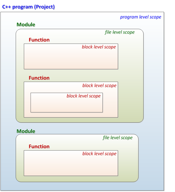
II.3.1.2. Lifetime of variables
A lifetime is a period of program execution where the given variable exists. On the basis of lifetime, identifiers can be divided into three groups: names of static, automatic and dynamic lifetime.
|
static lifetime |
Identifiers having a static or extern storage class have a static lifetime. The memory space allocated for static variables (and the data contained within it) remains until the end of program execution. A variable of this type is initialised once: when the program is launched. |
|
automatic lifetime |
Within blocks, variables defined without the static storage class and the parameters of functions have automatic (local) lifetime. The memory space of automatic lifetime variables (and the data contained within it) exist only in the block where they are defined. Variables with local lifetime are created on a new segment of memory each time their block is entered, and they are deleted when the block is exited (their content becomes lost). If a variable of this type is assigned an initial value, this initialization takes place every time the variable is created. |
|
dynamic lifetime |
Independently of their storage classes, memory blocks that are allocated by the operator new and deallocated by the operator delete have dynamic lifetime. |
II.3.1.3. Storage classes of block level variables
Variables that are defined within a function/program block or in the parameter list of functions are automatic (auto) by default. The keyword auto is not used in general. In addition, in the latest C++11 standard, this keyword has a new interpretation. Block level variables are often called local variables.
II.3.1.3.1. Automatic variables
Automatic variables are created when control is passed to their block and they are deleted when that block is exited.
As we have already said in previous chapters, compound statements (blocks) can be nested into each other. Each block can contain definitions (declarations) and statements in any order:
{
definitions, declarations and
statements
}
An automatic variable becomes temporarily inaccessible if another variable with the same name is defined in an inner block. So it is hidden until the end of that inner block and there is not any possibility to access the hidden (existing) variable:
int main()
{
double limit = 123.729;
// the value of the double type variable limit is 123.729
{
long limit = 41002L;
// the value of the long type variable limit is 41002L
}
// the value of the double type variable limit is 123.729
}
Since automatic variables cease to exist when the function containing them is exited, it is forbidden to create a function that returns the address or reference to a local variable. If we want to allocate space within a function for a variable that is used outside the function, then we should allocate that memory space dynamically.
In C++, loop variables defined in the header of a for loop are also automatic:
for (int i=12; i<23; i+=2) cout << i << endl; ↯ cout << i << endl; // compilation error: i is not defined
The initialization of automatic variables always takes place if control is passed to their block. However, it is only the variables defined with an initial value that receive an initial value. (The value of the other variables is undefined!).
II.3.1.3.2. The register storage class
The register storage class can only be used for automatic local variables and function parameters. If we provide the keyword register for a variable, we ask the compiler to create that variable in the register of the processor, if possible. In that way, the compiled code may be executed faster. If there is no free register for that purpose, the variable is created as an automatic variable. However, register variables are created in memory if the address operator (&) is used with them.
It should be noted that C++ compilers are able to optimize the compiled code, which results in general in a more efficient program code than if the keyword register was used. So it is not surely more efficient to use register storage classes.
The following Swap() function can be executed much faster than its previously presented version. (We use the word "can" because it is not known in advance how much register storage class specification takes into consideration the compiler.)
void Swap(register int &a, register int &b) {
register int c = a;
a = b;
b = c;
}
The function StrToLong() of the following example converts a decimal number stored in a string into a value of type long:
long StrToLong(const string& str)
{
register int index = 0;
register long sign = 1, num = 0;
// leaving out leading blanks
for(index=0; index < str.size()
&& isspace(str[index]); ++index);
// sign?
if( index < str.size()) {
if( str[index] == '+' ) { sign = 1; ++index; }
if( str[index] == '-' ) { sign = -1; ++index; }
}
// digits
for(; index < str.size() && isdigit(str[index]); ++index)
num = num * 10 + (str[index] - '0');
return sign * num;
}
The lifetime, visibility of register variables and the method of their initialization equal with those of variables having an automatic storage class.
II.3.1.3.3. Local variables with static lifetime
By using static storage classes instead of auto, we can create block level variables with static lifetime. The visibility of a variable like this is restricted to the block containing its definition; however, the variable exists from the time the program is launched until the program is exited. Since the initialization of static local variables takes place only once (when they are created), these variables keep their value even after the block is exited (between function calls).
The function Fibo() of the following example determines the next element of a Fibonacci sequence from the 3th element. Within the function, the static local variables a0 and a1 keep the value of the last two elements even after the block is exited.
#include <iostream>
using namespace std;
unsigned Fibo() {
static unsigned a0 = 0, a1 = 1;
unsigned a2 = a0 + a1;
a0 = a1;
a1 = a2;
return a2;
}
int main() {
for (register int i=2; i<10; i++)
cout << Fibo() << endl;
}
II.3.1.4. Storage classes of file level variables
Variables defined outside functions automatically have extern, i.e. program level scope. When software is developed from many modules (source files), it is not sufficient to use global variables in order that the principles of modular programming be observed. We might also need variables defined on module level: the access of these variables can be restricted to the source file (data hiding). This can be achieved by assigning extern variables a static storage class. If constants are defined outside functions, they have also internal linkage by default.
In the following program generating a Fibonacci sequence, the variables a0 and a1 were defined on a module level in order that their content remain accessible from another function (FiboInit()).
#include <iostream>
using namespace std;
const unsigned first = 0, second = 1;
static unsigned a0 = first, a1 = second;
void FiboInit() {
a0 = first;
a1 = second;
}
unsigned Fibo() {
unsigned register a2 = a0 + a1;
a0 = a1;
a1 = a2;
return a2;
}
int main() {
for (register int i=2; i<5; i++)
cout << Fibo() << endl;
FiboInit();
for (register int i=2; i<8; i++)
cout << Fibo() << endl;
}
The initialization of static variables takes place only once: when the program is launched. In case we do not provide an initial value for them in their definition, then the compiler initializes these variables automatically to 0 (by filling up its memory space with 0 bytes). In C++, static variables can be initialized by any expression.
C++ standards recommend using anonymous namespaces instead of static external variables (see later).
II.3.1.5. Storage classes of program level variables
Variables that are defined outside functions and to which a storage class is not assigned have an extern storage class by default. (Of course, the keyword extern can be used here, even if that is the default case.)
The lifetime of extern (global) variables begins with the launching and ends with the end of the program. However, there might be problems with visibility. A variable defined in a given module can only be accessed from another module, if the latter contains the declaration of that variable (for example by including its declaration file).
When using program level global variables, we have to pay attention whether we define or declare them. If a variable is used without a storage class specification outside functions, this means defining this variable (independently of the fact that it is provided an explicit initial value or not). On the contrary, assigning them extern explicitly can have two consequences: without initial value, they are declared , with initial value, they are defined . The following examples demonstrate what we have said so far:
|
Same definitions (only one of them can be used) |
Declarations |
|---|---|
|
double sum; double sum = 0; extern double sum = 0; |
extern double sum;
|
|
int vector[12]; extern int vector[12] = {0}; |
extern int vector[]; extern int vector[12]; |
|
extern const int size = 7; |
extern const int size; |
It should be kept in mind that global variables can be declared anywhere in a program but the effects of these declarations start from the place of the declaration until the end of the given scope (block or module). It is a frequent solution to store declarations in header files for each module and to include them at the beginning of every source file.
The initialization of global variables takes place only once when the program starts. In case we do not provide any initial value to them, then the compiler initializes these variables automatically to 0. In C++, global variables can be initialised by any expression.
It should be kept in mind that global variables should only be used with caution and only if they are really needed. Even in the case of a bigger program, only some central extern variables are allowed.
II.3.2. Storage classes of functions
Functions can only have two storage classes. Functions cannot be defined in a block; therefore a function cannot be created within another function!
The storage class of a function determines its accessibility. Therefore functions without a storage class or those defined with the extern storage class have program level scope. On the contrary, functions having a static storage class have file level scope.
We mean by the definition of a function the function itself, whereas a declaration of a function means its prototype. The following table summarizes the definitions and declarations of the function calculating the geometric mean of two numbers, in the case of both storage class.
|
Definitions (only one of them can be used) |
Prototypes |
|---|---|
double GeomMean(double a, double b)
{
return sqrt(a*b);
}
extern double GeomMean(double a, double b)
{
return sqrt(a*b);
}
|
double GeomMean(double, double); extern double GeomMean(double, double); |
static double GeomMean(double a, double b)
{
return sqrt(a*b);
}
|
static double GeomMean(double, double); |
Prototypes can be placed anywhere in a program code but their effects start from the place of declaration and ends at the end of the given scope (block or module). It is common to store prototypes for each module in separate header files that have to be included at the beginning of each concerned source file.
File and program level declarations and definitions are demonstrated by the following example code made up of two modules. The mathematical module provides the program with the mathematical constants, an "intelligent" Random() function and a function Sin() capable of calculating in degrees.
|
// |
// | |
#include <iostream>
using namespace std;
extern int Random(int);
double Sin(double);
int main() {
for (int i=0; i<5; i++)
cout << Random(12)<< endl;
cout << Sin(45) << endl;
extern const double e;
cout << e << endl;
}
|
#include <ctime>
#include <cstdlib>
#include <cmath>
using namespace std;
extern const double pi = asin(1)*2;
extern const double e = exp(1);
static double Degree2Radian(double);
static bool firstrnd = true;
int Random(int n) {
if (firstrnd) {
srand((unsigned)time(0));
firstrnd = false;
}
return rand() % n;
}
double Sin(double degree) {
return sin(Degree2Radian(degree));
}
static double Degree2Radian(double degree) {
return degree/180*pi;
}
|
II.3.2.1. Accessing the compiled C functions from within C++ source
C++ compilers complete the name we have given for a function in the object code with the letters of the types from the parameter list of the function. This solution named C++ linkage makes possible the possibilities presented earlier in this chapter (overloading, function template).
When C++ was born, C language had already existed for nearly ten years. It was rightful to claim that the algorithms of compiled object modules and Library functions developed for C programs would also be accessible from C++ programs. (Programs in C source code could therefore be implemented in C++ with slight modifications.) C compilers place function names without any modification in the object code (C linkage), so they are not accessible by the C++ declarations presented above.
To handle this problem, C++ contains the type modifier extern "C". If a function sqrt() coded in C is intended to be used from C++ source code, it should be declared as
extern "C" double sqrt(double a);
This modifier makes C++ compilers to use the habitual C name generation for the function sqrt(). As a consequence, C functions cannot be redefined (overloaded)!
In case more C functions are needed to be accessed from a C++ code, these functions should be grouped under one extern "C" :
extern "C" {
double sin(double a);
double cos(double a);
}
If the descriptions of the functions of a C library are contained in a separated declaration file, it should be worth the following method:
extern "C" {
#include <rs232.h>
}
We should also use the extern "C" declaration if functions written and compiled in C++ are intended to be accessed from a C program code.
It is also worth mentioning here that the main () function also has extern "C" linkage.
II.3.3. Modular programs in C++
The structure of the example code of the preceding part becomes more structured if we create for the MatModule.cpp file a header file named MatModule.h that describes the interface of the module. Using constants becomes also simpler if they are placed in the file level scope (static). According to what has been said so far, the content of the MatModule.h header file:
// MatModule.h
#ifndef _MATMODULE_H_
#define _MATMODULE_H_
#include <cmath>
using namespace std;
// file level definitions/declarations
const double pi = asin(1)*2;
const double e = exp(1);
static double Degree2Radian(double);
// program level declarations
int Random(int n);
double Sin(double degree);
#endif
Lines with green and bold characters contain preprocessing statements that guarantee that the content of the MatModule.h header file would be included exactly once in the module containing the line
#include "MatModule.h"
(The Section II.4, “Preprocessor directives of C++” provides readers with more information on the usage of preprocessors.)
Including the header file results in modifying the C++ modules:
|
// |
// | |
#include <iostream>
using namespace std;
#include "MatModul.h"
int main() {
for (int i=0; i<5; i++)
cout << Random(12)<< endl;
cout << Sin(45) << endl;
cout << e << endl;
}
|
#include <ctime>
#include <cstdlib>
using namespace std;
#include "MatModul.h"
static bool firstrnd = true;
int Random(int n) {
if (firstrnd) {
srand((unsigned)time(0));
firstrnd = false;
}
return rand() % n;
}
double Sin(double degree) {
return sin(Degree2Radian(degree));
}
static double Degree2Radian(double degree) {
return degree/180*pi;
}
|
C++ compilers compile each module separately and create separate object modules for them because all the identifiers of each module have to be known in advance by compilers. This can be realized by placing declarations/prototypes and definitions adequately. After compilation, it is the task of the linker software to build one executable program from the object modules by resolving extern linkages from the object modules themselves or from standard libraries.
Integrated development environments automatize compilation and linking by creating projects. The only task of programmers is to add to the project the already existing C++ source files. In general, if we use the Build command from the menu, the whole compilation process takes place.
The
GNU C++
compiler can be activated for compilation and for linking with the following command line command. It also makes the compiler create the Project.exe executable file:
g++ -o Project MainModul.cpp MatModul.cpp
II.3.4. Namespaces
Names (identifiers) used in the program are stored by C++ compilers in different places (on the basis of how they are used) that are called namespaces. Within a given namespace, stored names have to be unique but there may be identical names in different namespaces. Two identical names that are situated in the same scope but not in the same namespace designate different identifiers. C++ compilers differentiate between the following namespaces:
II.3.4.1. The default namespaces of C++ and the scope operator
In C language, variables and functions defined on the file level (as well as Standard library functions) can be found in the same common namespace. C++ enclose Standard library elements in the namespace called std whereas the other elements defined on a file level are contained within the global namespace.
In order to be able to refer the elements of a namespace, we have to know how to use the scope operator (::). We will talk more about the scope operator later in that book, so now we only show examples for two of its possible usages.
With the help of :: operator, we can refer names having file and program level scope (that is identifiers of the global namespace) from any block of a program.
#include <iostream>
using namespace std;
long a = 12;
static int b = 23;
int main() {
double a = 3.14159265;
double b = 2.71828182;
{
long a = 7, b;
b = a * (::a + ::b);
// the value of b is 7*(12+23) = 245
::a = 7;
::b = 29;
}
}
We also use the scope operator to access directly names defined in the namespace std :
#include <iostream>
int main() {
std::cout<<"C++ language"<<std::endl;
std::cin.get();
}
II.3.4.2. Creating and using user-defined namespaces
Bigger C++ source codes are in general developed by numerous programmers. The functionalities of C++ presented so far are not enough to avoid collision or conflict of global (program level) names. Introducing namespaces having a user-defined name gives a good solution for these problems.
II.3.4.2.1. Creating namespaces
In source files, namespaces can be created either outside function blocks or in header files. In case a compiler find more namespaces with the same name, it unifies their contents, thus it extends the namespace defined earlier. To select a namespace, we have to use the keyword namespace:
namespace myOwnNamespace {
definitions and declarations
}
When planning program level namespaces, it is worth differentiating the namespaces containing definitions from those which can be placed in header files and which contain only declarations.
#include <iostream>
#include <string>
// declarations
namespace nsexample {
extern int value;
extern std::string name;
void ReadData(int & a, std::string & s);
void PrintData();
}
// definitions
namespace nsexample {
int value;
std::string name;
void PrintData() {
std::cout << name << " = " << value << std::endl;
}
}
void nsexample::ReadData(int & a, std::string & s) {
std::cout << "name: "; getline(std::cin, s);
std::cout << "value: "; std::cin >> a;
}
If a function declared in a namespace is created outside that namespace, the name of the function has to be qualified by the name of its namespace (in our example nsexample::).
II.3.4.2.2. Accessing the identifiers of a namespace
The identifiers provided in the namespace called nsexample can be accessed from every module to which the version of that namespace containing the declarations is included. Identifiers of a namespace can be accessed in many ways.
Directly by using the scope operator:
int main() {
nsexample::name = "Sum";
nsexample::value = 123;
nsexample::PrintData();
nsexample::ReadData(nsexample::value, nsexample::name);
nsexample::PrintData();
std::cin.get();
}
Or by using the directive using namespace :
It is of course more comfortable to make accessible all names for the whole program with the directive using namespace:
using namespace nsexample;
int main() {
name = "Sum";
value = 123;
PrintData();
ReadData(value, name);
PrintData();
std::cin.get();
}
Or by providing using -declarations:
With the help of using-declarations, we make available only the necessary elements from those of the namespace. This is the solution to choose if there is a name conflict between certain identifiers of a namespace.
int PrintData() {
std::cout << "Name conflict" << std::endl;
return 1;
}
int main() {
using nsexample::name;
using nsexample::value;
using nsexample::ReadData;
name = "Sum";
value = 123;
nsexample::PrintData();
ReadData(value, name);
PrintData();
std::cin.get();
}
II.3.4.2.3. Nested namespaces, namespace aliases
C++ makes it possible to create new namespaces within namespaces, that is to nest them in each other (nested namespaces). This procedure makes it possible to organize global names into a structured system. As an example, let's see the namespace called Project in which we define separate functions for every processor family!
namespace Project {
typedef unsigned char byte;
typedef unsigned short word;
namespace Intel {
word ToWord(byte lo, byte hi) {
return lo + (hi<<8);
}
}
namespace Motorola {
word ToWord(byte lo, byte hi) {
return hi + (lo<<8);
}
}
}
The elements of the namespace Project can be accessed in many ways:
using namespace Project::Intel;
int main() {
cout << hex;
cout << ToWord(0xab,0x12)<< endl; // 12ab
}
// -------------------------------------------------------
int main() {
using Project::Motorola::ToWord;
cout << hex;
cout << ToWord(0xab,0x12)<< endl; // ab12
}
// -------------------------------------------------------
using namespace Project;
int main() {
cout << hex;
cout << Intel::ToWord(0xab,0x12)<< endl; // 12ab
cout << Motorola::ToWord(0xab,0x12)<< endl; // ab12
}
// -------------------------------------------------------
int main() {
cout<<hex;
cout<<Project::Intel::ToWord(0xab,0x12)<< endl; // 12ab
cout<<Project::Motorola::ToWord(0xab,0x12)<<endl; // ab12
}
Accessing the elements of complex and multiple nested namespaces with long complex names (the elements of which are separated from each other by the namespace operator) makes program codes less legible. In order to solve this problem, C++ introduced the notion of namespace aliases:
namespace alias =externalNS::internalNS … ::most_internal_NS;
If we use aliases, the example above becomes much simpler:
int main() {
namespace ProcI = Project::Intel;
namespace ProcM = Project::Motorola;
cout << hex;
cout << ProcI::ToWord(0xab,0x12)<< endl; // 12ab
cout << ProcM::ToWord(0xab,0x12)<< endl; // ab12
}
II.3.4.2.4. Anonymous namespaces
C++ standards do not support the usage of the keyword static either in file level scopes or in namespaces. In module level scopes, we can create variables and functions in anonymous namespaces that are not accessible from outside of the compilation unit. However, the identifiers of anonymous namespaces can be used without restrictions within a module.
Within the same module, many anonymous namespaces can be created:
#include <iostream>
#include <string>
using namespace std;
namespace {
string password;
}
namespace {
bool ChangePassword() {
bool success = false;
string old, new1, new2;
cout << "Previous password: "; getline(cin, old);
if (password == old) {
cout << "New Password: "; getline(cin, new1);
cout << "New Password: "; getline(cin, new2);
if (new1==new2) {
password = new1;
success = true;
}
}
return success;
} // ChangePassword()
}
int main() {
password = "qwerty";
if (ChangePassword())
cout << "Successful password change!" << endl;
else
cout << "Not a successful password change!" << endl;
}
II.4. Preprocessor directives of C++
All C and C++ compilers contain a so-called preprocessor, which do not know anything about C++ language. Its only task is to create a program module completely in C++ from the source files of a computer program by carrying out word-processing operations. Consequently, a C++ compiler does not compile the source code programmers write but it processes the text the preprocessor creates (see Figure II.8, “The compilation process in C++”). It can clearly be deduced from that that finding program errors that result from the statements of the preprocessor is not an easy task.
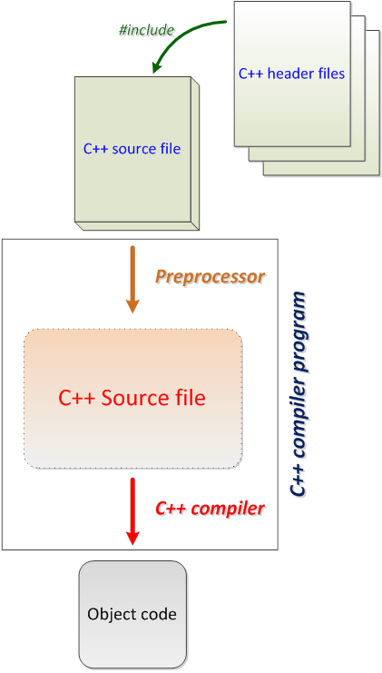
In most C++ compilers, preprocessing and real compilation are not separated from each other, that is the output of the preprocessor is not stored in any text file. (It should not be forgotten that the g++ compiler of C++ carries out only preprocessing if it is used by the switch –E .)
Actually, a preprocessor is a text processing software that is line-oriented and that can be programmed in a macro language. The rules of C++ language do not applied to the preprocessor:
the directives of the preprocessor are based on stricter rules than C++ statements (a single line can only contain one directive and directives cannot extend across more than one line unless this extension is not marked at the end of the line),
all operations carried out by the preprocessor are proper text processing tasks (independently of the fact that they may contain C++ keywords, expressions or variables).
The directives of the preprocessor start with a hash sign (#) at the beginning of the line. The most frequent operations that they carry out are: text replacement ( #define ), including a text file ( #include ) or keeping certain parts of the code under certain conditions ( #if ).
C++ relies completely on the features of the preprocessor directives of C. Since preprocessing is out of the scope of compilers of the strictly typed C++ language, C++ attempts to reduce the need of using preprocessors to a minimal level by introducing new solutions. In a C++ code, some preprocessor directives can be replaced with C++ solutions: instead of using #define constants, one can use constants of type const; instead of using #define macros , one can write inline function templates.
II.4.1. Including files
When the preprocessor encounters an #include directive, the content of the file figuring in the directive is integrated (inserted) in the code in the place of the directive. Generally, it is header files containing declarations and preprocessor directives that are integrated in the beginning of the code; however, inclusion can be applied to any text file.
#include <header> #include "filepath"
The first form is used to include the standard header files of C++ from the folder named include of the development kit:
#include <iostream> #include <cmath> #include <cstdlib> #include <ctime> using namespace std;
The second form is used to include non-standard files from the folder storing the actual C++ module or from any other folder:
#include "Module.h" #include "..\Common.h"
The following table sums up the keywords and language elements that can be used in header files:
|
C++ elements |
Example |
|---|---|
|
Comments |
|
|
Conditional directives |
|
|
Macro definitions |
|
|
#include directives |
|
|
Enumerations |
|
|
Constant definitions |
|
|
Namespaces having an identifier |
|
|
Name declarations |
|
|
Type definitions |
|
|
Variable declarations |
|
|
Function prototypes |
|
|
inline function definitions |
|
|
template declarations |
|
|
template definitions |
|
The following elements should never be placed in include files:
definitions of non-inline functions,
variable definitions,
definitions of anonymous namespaces.
One part of the elements that can be placed in a header file have to be included only once in a code. That is why, all header files have to have a special preprocessing structure based on conditional directives:
// Module.h
#ifndef _MODULE_H_
#define _MODULE_H_
the content of the header file
#endif
II.4.2. Conditional compilation
By using conditional directives, one can achieve that certain parts of a source code would be inserted into the C++ program created by the preprocessor only if given conditions are fulfilled. The code parts to be compiled under conditions can be selected in many ways, by using the following preprocessor directives: #if, #ifdef, #ifndef, #elif, #else and #endif.
In an #if statement, the condition can be expressed by a constant expression. If the value of the latter is zero, it means false; if the latter has a value other than 0, that means true. In an expression, only the following elements are allowed: integer and character constants, operations of type defined.
#if 'O' + 29 == VALUE
In a condition, we can check whether a symbol is defined or not with the help of the operator named defined. This operator returns 1, if its operand exists. Otherwise it returns 0:
#if defined symbol #if defined(symbol)
Since checkings of this kind are often used, we can test whether a symbol exists or not with separate preprocessing statements:
#ifdef symbol #if defined(symbol) #ifndef symbol #if !defined(symbol)
More complex conditions can be checked by #if:
#if 'O' + 29 == VALUE && (!defined(NAME) || defined(NUMBER))
The following simple text makes the code part enclosed within the #if and #endif lines integrated in the compilation unit:
#if constant_expression
code part
#endif
This structure can well be used to integrate information into a source code in order that debugging become simpler. In that example, if the value of the symbol TEST is 1, this complementary information gets compiled in the code, and if it is 0, this information is not enabled:
#define TEST 1
int main() {
const int size = 5;
int array[size] = { 12, 23, 34, 45, 56 };
int i;
for (int i = 0; i < size; i++) {
array[i] *= 2;
#if TEST != 0
cout << "i = " << i << endl;
cout << "\tarray[i] = " << array[i] << endl;
#endif
}
}
Instead of the structure above, it is better to use a solution that examines the definition of the symbol TEST. For that purpose, TEST can be defined without a value, which can be assigned to it from a parameter of the compiler:
#define TEST
int main() {
const int size = 5;
int array[size] = { 12, 23, 34, 45, 56 };
int i;
for (int i = 0; i < size; i++) {
array[i] *= 2;
#if defined(TEST)
cout << "i = " << i << endl;
cout << "\tarray[i] = " << array[i] << endl;
#endif
}
}
Each pair of the following checkings return the same results:
#if defined(TEST) ... // defined #endif |
#ifdef TEST ... // defined #endif | |
#if !defined(TEST) ... // not defined #endif |
#ifndef TEST ... // not defined #endif |
If the following structure is used, we can choose between two code parts:
#if constant_expression
codepart1
#else
codepart2
#endif
The following example creates the two-dimensional array named array depending on the value of the symbol SIZE:
#define SIZE 5
int main() {
#if SIZE <= 2
int array[2][2];
const int size = 2;
#else
int array[SIZE][SIZE];
const int size = SIZE;
#endif
}
For more complex structures, it is recommended to use multi-way branches.
#if constant_expression1
codepart1
#elif constant_expression2
codepart2
#else
codepart3
#endif
The following example integrates the declaration file on the basis of the manufacturer:
#define IBM 1
#define HP 2
#define DEVICE IBM
#if DEVICE == IBM
#define DEVICE_H "ibm.h"
#elif DEVICE == HP
#define DEVICE_H "hp.h"
#else
#define DEVICE_H "other.h"
#endif
#include DEVICE_H
II.4.3. Using macros
The most controversial domain about using preprocessors is the usage of #define macros in C++ programs. The reason for that is that the result of processing the macro may not always correspond to the expectations of programmers. Macros are widely used in codes written in C, but they have less importance in C++. The definition of the C++ programming language prefers const and inline function templates to macros. In the present section, we will always prefer a secure macro usage.
The #define directive is used to assign an identifier to C++ constants, keywords and frequently used statements and expressions. The symbols defined for preprocessors are called macros. In a C++ source code, it is recommended that macro names should be completely written in upper-case letters in order that they become visibly separated from C++ identifiers used in the code.
Preprocessors check the source code line by line whether it contains an already defined macro name. If yes, they replace it with the appropriate replacement text and then they check again the line for further macros, which may be followed by further replacements. This process is called macro replacement or macro substitution. Macros are created by a #define statement and deleted by the directive named #undef .
II.4.3.1. Symbolic constants
Symbolic constants can be created by using the simple form of the #define directive:
#define identifier #define identifier replacement_text
Let's see some examples how to define and use symbolic constants.
#define SIZE 4
#define DEBUG
#define AND &&
#define VERSION "v1.2.3"
#define BYTE unsigned char
#define EOS '\0'
int main() {
int v[SIZE];
BYTE m = SIZE;
if (m > 2 AND m < 5)
cout << "2 < m < 5" << endl;
#ifdef DEBUG
cout << VERSION << endl;
#endif
}
The source file after the preprocessing (replacements) is the following:
int main() {
int v[4];
unsigned char m = 4;
if (m > 2 && m < 5)
cout << "2 < m < 5" << endl;
cout << "v1.2.3" << endl;
}
In the previous example, some symbolic constants can be replaced by identifiers of types const and typedef in C++:
#define DEBUG
#define AND &&
const int size = 4;
const string version = "v1.2.3";
const char eos = '\0';
typedef unsigned char byte;
int main() {
int v[size];
byte m = size;
if (m > 2 AND m < 5)
cout << "2 < m < 5" << endl;
#ifdef DEBUG
cout << version << endl;
#endif
}
II.4.3.2. Parameterized macros
The macros can be efficiently used in much more cases if they are parameterized. The general form of a function-like parameterized macro:
#define identifier(parameter_list) replacement_text
Using (calling) a macro:
identifier(argument_list)
The number of the arguments in a macro call has to be identical with that of the parameters in the definition.
In order that parameterized macros work securely, the following two rules have to observed:
The parameters of a macro always have to be enclosed within parentheses in the body of the macro (in the replacement text).
Increment (++) and decrement (--) operators should not be used in the argument list when the macro is called.
The following example code demonstrates some frequently used macro definitions and the way they can be called:
// determining the absolute value of x
#define ABS(x) ( (x) < 0 ? (-(x)) : (x) )
// calculating the maximum value of a and b
#define MAX(a,b) ( (a) > (b) ? (a) : (b) )
// calculating the square of X
#define SQR(X) ( (X) * (X) )
// generating a random number within a given interval
#define RANDOM(min, max) \
((rand()%(int)(((max) + 1)-(min)))+ (min))
int main() {
int x = -5;
x = ABS(x);
cout << SQR(ABS(x));
int a = RANDOM(0,100);
cout << MAX(a, RANDOM(12,23));
}
The backslash (\) character at the end of the first line of the macro named RANDOM() indicates that the definition of that macro is continued in the next line. The content of the main () function cannot be qualified as legible at all after the preprocessing process:
int main() {
int x = -5;
x = ( (x) < 0 ? (-(x)) : (x) );
cout << ( (( (x) < 0 ? (-(x)) : (x) )) *
(( (x) < 0 ? (-(x)) : (x) )) );
int a = ((rand()%(int)(((100) + 1)-(0)))+ (0));
cout << ( (a) > (((rand()%(int)(((23) + 1)-(12)))+ (12)))
? (a) : (((rand()%(int)(((23) + 1)-(12)))+ (12))) );
}
All advantages of macros (type-independence, faster code) can be achieved by using inline functions/function templates (instead of macros) while keeping the C++ code legible:
template <class tip> inline tip Abs(tip x) {
return x < 0 ? -x : x;
}
template <class tip> inline tip Max(tip a, tip b) {
return a > b ? a : b;
}
template <class tip> inline tip Sqr(tip x) {
return x * x;
}
inline int Random(int min, int max) {
return rand() % (max + 1 - min) + min;
}
int main() {
int x = -5;
x = Abs(x);
cout << Sqr(Abs(x));
int a = Random(0,100);
cout << Max(a, Random(12,23));
}
II.4.3.3. Undefining a macro
A macro can be undefined anytime and can be redefined again, even with a different content. It can be undefined by using the #undef directive. Before redefining a macro with a new content, the old definition always has to be undefined. The #undef statement does not signal an error if the macro to be undefined does not exist:
#undef identifier
The following example code traces the functioning of #define and #undef statements:
|
Original source code |
Substituted code |
|---|---|
int main() {
#define MACRO(x) (x) + 7
int a = MACRO(12);
#undef MACRO
a = MACRO(12);
#define MACRO 123
a = MACRO
}
|
int main() {
int a = (12) + 7;
a = MACRO(12);
a = 123
}
|
II.4.3.4. Macro operators
In our previous examples, replacement was carried out by the preprocessor only in case of separate parameters. There are cases where a parameter is a part of an identifier or where the value of an argument is to be reused as a string. If replacement has to be done in these cases as well, then the macro operators ## and # have to be used.
If the # character is placed before the parameter in a macro, the value of the parameter is replaced as enclosed within quotation marks (i.e. as a string). With this method, replacement can be carried out on strings as well, since the compiler will concatenate the string literals standing one after another into one string constant. The following code prints out the name and value of any variable by using the macro named INFO():
#include <iostream>
using namespace std;
#define INFO(variable) \
cout << #variable " = " << variable <<endl;
int main() {
unsigned x = 23;
double pi = 3.14259265;
string s = "C++ language";
INFO(x);
INFO(s);
INFO(pi);
}
x = 23 s = C++ language pi = 3.14259 |
By using the ## operator, two syntactic units (tokens) can be concatenated. To achieve this, the ## operator has to be inserted between the parameters in the body of a macro.
In the following example, the macro named PERSON() populates the array named people with values of structure type:
#include <string>
using namespace std;
struct person {
string name;
string info;
};
string Ivan_Info ="K. Ivan, Budapest, 9";
string Alice_Info ="O. Alice, Budapest, 33";
#define PERSON(NAME) { #NAME, NAME ## _Info }
int main(){
person people[] = {
PERSON (Ivan),
PERSON (Alice)
};
}
The content of the main () function after preprocessing:
int main(){
person people[] = {
{ "Ivan", Ivan_Info },
{ "Alice", Alice_Info }
};
}
There are cases when one macro is not sufficient for a given purpose. In the following example, the version number is created by concatenating the given symbolic constants:
#define MAJOR 7 #define MINOR 29 #define VERSION(major, minor) VERSION_MINOR(major, minor) #define VERSION_MINOR(major, minor) #major "." #minor static char VERSION1[] = VERSION(MAJOR,MINOR); // "7.29" static char VERSION2[] = VERSION_MINOR(MAJOR,MINOR); //"MAJOR.MINOR"
II.4.3.5. Predefined macros
ANSI C++ standard contains the following predefined macros. (Almost all identifiers start and end with a double underscore character.) The name of predefined macros cannot be used in #define and #undef statements. The value of predefined macros can be integrated into the text of a code but can also be used as a condition in conditional directives.
|
Macro |
Description |
Example |
|---|---|---|
|
|
String constant containing the date of the compilation. |
|
|
|
String constant containing the time of the compilation. |
|
|
|
The date and time of the last modification of the source file in a string constant" |
|
|
|
String constant containing the name of the source file. |
|
|
|
A numeric constant, containing the number of the actual line of the source file (numbering starts from 1). |
|
|
|
Its value is 1 if the compiler works as an ANSI C++, otherwise it is not defined. | |
|
|
Its value is 1, if its value is tested in a C++ source file, otherwise it is not defined. |
II.4.3.6. #line, #error and #pragma directives
There are a lot of utility software that transforms a code written in a special programming language to a C++ source file (program generators).
The #line directive forces C++ compilers not to signal the error code in the C++ source text but in the original source file written in another special language. (The code and file name set by a #line statement are also present in the value of the symbols __LINE__ and __FILE__ .)
#line beginning_number #line beginning_number "filename"
If it is inserted in a code, an #error directive can be used to print out a compilation error message which contains the text provided in the statement:
#error error_message
In the following example, compilation ends with an error message if we do not use the C++ mode:
#if !defined(__cplusplus)
#error Compilation can only be carried out in C++ mode!
#endif
#pragma directives are used to control the compilation process in an implementation-dependent way. (There are not any standard solution for this directive.)
#pragma instruction
If the compiler encounters an unknown #pragma instruction, it does not consider that. Therefore the portability of computer programs is not endangered by this directive. For example, the alignment of structure members to different boundaries and disabling the printing out of warning compilation messages having a specific index can be done in the following way:
#pragma pack(8) // aligned to 8 byte boundary #pragma pack(push, 1) // aligned to 1 byte boundary #pragma pack(pop) // aligned again to 8 byte boundary #pragma warning( disable : 2312 79 )
The empty directive (#) can also be used, but it does not affect preprocessing:
#
Chapter III. Object-oriented programming in C++
- III.1. Introduction to the object-oriented world
- III.2. Classes and objects
- III.3. Inheritance (derivation)
- III.4. Polymorphism
- III.5. Class templates
- III.5.1. A step-be-step tutorial for creating and using class templates
- III.5.2. Defining a generic class
- III.5.3. Instantiation and specialisation
- III.5.4. Value parameters and default template parameters
- III.5.5. The "friends" and static data members of a class template
- III.5.6. The Standard Template Library (STL) of C++
Object-oriented programming (OOP) is a contemporary programming methodology (paradigm), which divides whole programs into closed program units (objects) that have individual features and that are able to function by themselves. Object-oriented programming offers a much more efficient solution to most problems than classic, structured programming and it can reduce the time necessary to develop software by supporting the creation and reuseability of objects doing abstract operations.
III.1. Introduction to the object-oriented world
Object-oriented programming uses the "things" ("objects") and the interaction between them to plan and to develop applications and computer programs. This methodology comprises solutions, like encapsulation, modularity, polymorphism and inheritance.
It should be noted that OOP languages only offer tools and support in order that object-orientation be realised. In the present book, we will also focus on presenting these tools after a short overview.
III.1.1. Basics
Now let's have a look at the basic notions of object-orientation. To understand these, we do not even have to have much knowledge in programming.
Class
A class determines the abstract features of a thing (object), including its features (attributes, fields, properties) and its behaviour (what the thing can do, methods, operations and functions).
We can say that a class is a scheme describing the nature of something. For example, the class Truck has to contain the common properties of trucks (manufacturer, engine, brake system, maximum load etc.), as well as their specific behaviour, like braking, turning to left etc.
Classes offer by themselves modularity and structuredness for object-oriented computer programs. The notion of class should also be understandable for those people who are familiar with the given problem but not familiar with programming that is the features of a class should be expressive. The code of a class should be relatively independent (encapsulation). Both the integrated properties and the methods of a class are called class members (data member and member function in C++).
Object
An object is a scheme (an example) of a class. With the help of the class Truck, we can define all possible trucks by enumerating their properties and behaviour forms. For example, the class Truck has the feature brake system, but the brake system of the object myCar can be an electronically controlled one (EBS) or a simple air brake.
Instance
The notion of instance (of a class) is synonymous with the notion of object. Instance means an actual object created at runtime. So, myCar is an instance of the class Truck. The set of the property values of the actual object is called the state of that object. Therefore all objects are characterised by the state and behaviour defined in their corresponding class.
Method
Methods are responsible for the capabilities of objects. In spoken language, the corresponding term for methods is verbs. Since myCar is a Truck, it has the ability of braking, so Brake() is one of the methods of myCar. Of course, it may have other methods as well, like Ignition(), StepOnTheGas(), TurnLeft() or TurnRight(). Within a program, a method has only effect on the given object in general when it is used. Although all trucks can brake, activating (calling) the method Brake() will only slow down one given vehicle. In C++, methods are rather called member functions.

Message passing
Message passing is the process during which an object sends data to another object or "asks" another object to execute one of its methods. The role of message passing can be better understood if we think of the simulation of the functioning of trucks. In that simulation, the object driver sends a "brake" message to activate the Brake() method of myCar, which results in braking the vehicle. The syntax of message passing may be very different among different programming languages. On the code level, message passing is realised by calling a method in C++.
III.1.2. Basic principles
The object-orientation of a system, of a programming language can be measured by supporting the following principles. If it is only some of these principles that are realised, that is an object-based system, if all four principles are supported, that is an object-oriented system.
III.1.2.1. Encapsulation, data hiding
As we have already seen, classes principally consist of features (state) and methods (behaviour). However, the state and behaviour of objects can be divided into two groups. There are some features and methods that we hide from other objects. These are internal (private or protected) states and behaviour. However, the others are made public. According to the basic principles of OOP, the state features have to be private while most of the methods may be public. If it is needed, public methods can be used to access private features in a controlled way.
It is not necessary for an object that passes a message to another object to know the inner structure of the latter. For example, the Truck has the method Brake(), which exactly defines how braking takes place. However, the driver of myCar does not have to know how that car brakes.
All objects provide a well-defined interface for the external world. That interface defines what can be accessed from the given object from the outside. If this interface is completely written, there is not any problem to modify the internal world of the class in the future for client applications using that object. For example, it can be ensured that trailers may only be connected to objects of the class HeavyTruck.
III.1.2.2. Inheritance
Inheritance means creating specific versions of a class that inherit the features and behaviour of their parent class (base class) and use them as if they were of their own. The classes created in this way are called subclasses or derived classes.
For example, the subclasses Van and HeavyTruck are derived from the class Truck. In the following, myCar will be an instance of the class HeavyTruck. Let's also suppose that the class Truck defines the method Brake() and the property brake system. All classes derived from that class (Van and HeavyTruck) inherit these members, so programmers have to write only once the code corresponding to them.
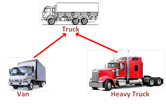
Subclasses may change the inherited properties. For example, the class Van can prescribe that its maximum load is 20 tons. The subclass HeavyTruck may make EBS braking as its default for its method Brake().
Derived classes can be extended with new members as well. The method Navigate() can be added to the class HeavyTruck. On the basis of what has been said so far, the method Brake() of the given instance HeavyTruck uses an EBS-based brake in spite of the fact that it inherits a traditional Brake() method from the class Truck; it also has a new method named Navigate(), which cannot be found in the class Van.
Actually, inheritance is an is-a relation: myCar is a HeavyTruck, a HeavyTruck is a Truck. So myCar has the methods of both HeavyTruck and Truck.
Both derived classes have one direct parent class, namely Truck. This inheritance method is called single inheritance to be differentiated from multiple inheritance.
Multiple inheritance means that a derived class inherits the members of more direct parent classes. For example, we can define two classes totally independent of each other with the names Truck and Ship. From these classes, we can create a new class named Amphibious, which has the features and behaviour of both trucks and ships. Most programming languages (ObjectPascal, Java, C#) support only single inheritance; however, C++ offers both inheritance methods.
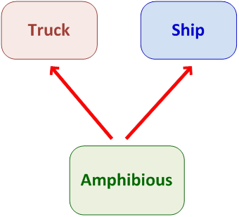
III.1.2.3. Abstraction
Abstraction simplifies complex reality by modelling problems with their corresponding classes and it has its effects on the level of inheritance appropriate for these problems. For example, myCar can be treated as a Truck in most cases; however, it may also be a HeavyTruck as well if the specific features and behaviour of HeavyTruck are needed but it can also be considered as a Vehicle if it is treated as a member of a fleet of vehicles. (Vehicle is the parent class of Truck in the example.)
Abstraction can be achieved through composition. For example, a class named Car has to contain the components engine, gearbox, steering gear and many others. In order to construct a Car, we do not have to know how the different components work, we only have to know how to connect to them (i.e. its interface). An interface determines how to send them or receive from them messages and it gives information about the interaction between the components of the class.
III.1.2.4. Polymorphism
Polymorphism makes it possible to replace the content of some inherited (deprecated) behaviour forms (methods) with a new one in the derived class and to treat the new, replaced methods as the members of the parent class.
For the next example, let's suppose that the classes Truck and Bicycle inherit the method Accelerate() of the class Vehicle. In the case of a Truck, the command Accelerate() means the operation StepOnTheGas(), whereas in the case of a Bicycle it means calling the method Pedal(). In order that acceleration function correctly, the method Accelerate() of the derived classes should override the method Accelerate() inherited from the class Vehicle. This is overriding polymorphism.
Most OOP languages support parametric polymorphism as well where methods are written for compilers as schemes independently of types. In C++, this can be carried out with templates.
III.1.3. An object-oriented example code
Finally, let's see a C++ code written on the basis of the things said so far. Now, we mainly aim at giving readers some impressions about OOP, since OOP is only detailed in the following subchapters of the present book.
#include <iostream>
#include <string>
using namespace std;
class Truck {
protected:
string manufacturer;
string engine;
string brake_system;
string maximum_load;
public:
Truck(string ma, string en, string brake,
double load) {
manufacturer = ma;
engine = en;
brake_system = brake;
maximum_load = load;
}
void StartUp() { }
void StepOnTheGas() { }
virtual void Brake() {
cout<<"Classic braking."<< endl;
}
void TurnLeft() { }
void TurnRight() { }
};
class Van : public Truck {
public:
Van(string ma, string en, string brake)
: Truck(ma, en, brake, 20) { }
};
class HeavyTruck : public Truck {
public:
HeavyTruck(string ma, string en, string brake, double load)
: Truck(ma, en, brake, load) { }
void Brake() { cout<<"Brake with EBS."<< endl; }
void Navigate() {}
};
int main() {
Van post("ZIL", "Diesel", "airbrake");
post.Brake(); // Classic braking.
HeavyTruck myCar("Kamaz", "gas engine", "EBS", 40);
myCar.Brake(); // Brake with EBS.
}
The following chapters of this book presents the C++ tools that realise the solutions related to the notions presented above. However, this overview is not enough for acquiring a routine in OOP, it only helps getting started.
III.2. Classes and objects
In C++ language, there are two possibilities to create an ADT – abstract data type of the object-oriented framework. The type struct of C++ is an extension to the structure type of C language and as such, it has become able to define abstract data types. C++ also offers us the new class type.
The types struct and class are built up of data members and related operations (member functions). Classes can be created by both data types; however, it is the class type that observes more the principles of obejct- orientation because of the default access restriction of its members. By default, all members of a type struct is public, whereas the members of a type class can only be accessed by the member functions of that class.
A class declaration has two parts. The header of the class contains the keyword class/struct, followed by the name of the class. The header is followed by the class body, which is enclosed within curly brackets followed by a semi-colon. Declarations contain not only data members and member functions but also keywords regulating access to the members and followed by a colon: public, private (hidden) and protected.
class ClassName {
public:
type4 Function1(parameterlist1) { }
type5 Function2(parameterlist2) { }
protected:
type3 data3;
private:
type1 data11, data12;
type2 data2;
};
The declaration of class and struct classes can be placed anywhere in a C++ code where a declaration is allowed; however what comply the most with contemporary software development methods is a declaration on a module (file) level.
III.2.1. From structures to classes
In this chapter, based on our previous knowledge about the type struct, we will learn how to create and use objects. The problems raised in the subchapters are first solved in a conventional way than in an object-oriented aspect.
III.2.1.1. A little revision
We have already learnt how to group the data necessary to solve a problem with a structure type if the data are to be stored in the members of that structure:
struct Employee{
int employeeID;
string name;
float salary;
};
We are also able to define operations with functions that get as an argument the structure type variable:
void IncreaseSalary(Employee& a, float percent) {
a.salary *= (1 + percent/100);
}
The members of the structure can be accessed by the dot or arrow operator depending on who we entrust with memory allocation: ourselves or compilers:
int main() {
Employee engineer;
engineer.employeeID = 1234;
engineer.name = "Tony Clever";
engineer.salary = 2e5;
IncreaseSalary(engineer,12);
cout << engineer.salary << endl;
Employee *pAccountant = new Employee;
pAccountant->employeeID = 1235;
pAccountant->name = "Sarah Rich";
pAccountant->salary = 3e5;
IncreaseSalary(*pAccountant,10);
cout << pAccountant->salary << endl;
delete pAccountant;
}
Of course, structured and efficient program codes can be created in this way too; however, in this chapter, we intend to go further.
III.2.1.2. Grouping together data and operations
As a first step, relying on the basis of the principle named encapsulation, we group together data and operations to be done on them in one code unit, which we call class.
struct Employee {
int employeeID;
string name;
float salary;
void IncreaseSalary(float percent) {
salary *= (1 + percent/100);
}
};
It can be seen at first glance, that the function IncreaseSalary() does not receive the class type variable (object) as a parameter, since it carries out an operation on the object by default. The main () function that demonstrates the usage of the objects of type Employee, since we only call now the member function corresponding to the variable:
int main() {
Employee engineer;
engineer.employeeID = 1234;
engineer.name = "Tony Clever";
engineer.salary = 2e5;
engineer.IncreaseSalary(12);
cout << engineer.salary << endl;
Employee *pAccountant = new Employee;
pAccountant->employeeID = 1235;
pAccountant->name = "Sarah Rich";
pAccountant->salary = 3e5;
pAccountant->IncreaseSalary(10);
cout << pAccountant->salary << endl;
delete pAccountant;
}
III.2.1.3. Data hiding
Accessing class type variables (objects) directly contradicts the principle of data hiding. In object-oriented programming it is required that the data members of classes could not be accessed directly from the outside. The type struct offers complete access to its members by default, whereas the class type completely hides its members from the outside, which complies much more with the principles of OOP. It should be noted that the access of class elements can be defined by programmers as well with the keywords private, protected and public.
public members can be accessed anywhere within the code where the object itself is accessible. On the contrary, private members can be accessed only from the the member functions of their class. (The access type protected will be applied in the case of inheritance treated in Chapter Section III.3, “Inheritance (derivation)”
Within a class, a member group of any number of elements can be created with the usage of the keywords (private, protected, public) and there is no restriction on the order of groups.
If we stick to the previous example, it is necessary to write further member functions with which we can set and get in a controlled way the value of data members because of their restricted access modes. The setting functions may also check that only valid data could appear in the object of type Employee. Getting functions are often defined as a constant, which means that the value of data members cannot be modified with that function. In a constant member function, the reserved word const is put between the header and the body of that function. In our example, GetSalary() is a constant member function.
class Employee{
private:
int employeeID;
string name;
float salary;
public:
void IncreaseSalary(float percent) {
salary *= (1 + percent/100);
}
void SetData(int code, string n, float s) {
employeeID = code;
name = n;
salary = s;
}
float GetSalary() const {
return salary;
}
};
int main() {
Employee engineer;
engineer.SetData(1234, "Tony Clever", 2e5);
engineer.IncreaseSalary(12);
cout << engineer.GetSalary() << endl;
Employee *pAccountant = new Employee;
pAccountant->SetData(1235, "Sarah Rich", 3e5);
pAccountant->IncreaseSalary(10);
cout << pAccountant->GetSalary() << endl;
delete pAccountant;
}
It should be noted that data members can be changed with the help of constant member functions, too, in case they are declared with the keyword mutable, for example:
mutable float salary;
However, these solutions are rarely used.
It should be noted that if all data members of a class have public access, the object can be initialised by the solution already presented in the case of structures, for example:
Employee doorman = {1122, "John Secure", 1e5};
Since the useability of the formula above will be later restricted by other constraints as well (it should not be a derived class, it cannot have virtual member functions), it is recommended that they be initialised by the special member functions of classes, namely by the so-called constructors.
III.2.1.4. Constructors
In program codes using classes, one of the most frequent operations is creating objects. Some objects are created by programmers themselves by static or dynamic memory allocation (see example above); however, there are cases when the compiler creates so-called temporary object instances. How can we assign the data members of objects to be created an initial value? By data members that are called constructors.
class Employee{
private:
int employeeID;
string name;
float salary;
public:
Employee() { // default
employeeID = 0;
name = "";
salary = 0;
}
Employee(int code, string n, float s) { // by parameters
employeeID = code;
name = n;
salary = s;
}
Employee(const Employee & a) { // by copying values
employeeID = a.employeeID;
name = a.name;
salary = a.salary;
}
void IncreaseSalary(float percent) {
salary *= (1 + percent/100);
}
void SetName(string n) {
name = n;
}
float GetSalary() const {
return salary;
}
};
int main() {
Employee employee;
employee.SetName("Stephen Smith");
Employee engineer(1234, "Tony Clever", 2e5);
engineer.IncreaseSalary(12);
cout << engineer.GetSalary() << endl;
Employee firstEngineer = engineer;
// or: Employee firstEngineer(engineer);
firstEngineer.IncreaseSalary(50);
cout << firstEngineer.GetSalary() << endl;
Employee *pEmployee = new Employee;
pEmployee->SetName("Stephen Smith");
delete pEmployee;
Employee *pAccountant;
pAccountant = new Employee(1235, "Sarah Rich", 3e5);
pAccountant->IncreaseSalary(10);
cout << pAccountant->GetSalary() << endl;
delete pAccountant;
Employee *pFirstEngineer=new Employee(engineer);
pFirstEngineer->IncreaseSalary(50);
cout << pFirstEngineer->GetSalary() << endl;
delete pFirstEngineer;
}
In the example above, we created a constructor without parameters, a constructor with parameters and a copy constructor, making use of function name overloading. Thus, a constructor is a member function the name of which corresponds to the name of the class and has no return type. The constructor of a class is called automatically by compilers every time an object of the given class is created. A constructor has no return value. Except from that, it behaves like any other member function. With redefined (overloaded) constructors, an object can be initialised in many ways.
A constructor does not allocate memory space for the object to be created, it only has to initialise the memory space already allocated for it. However, if the object contains a pointer, then the constructor has to ensure that a memory space to which the pointer points is allocated.
A class has two constructors by default: a constructor without parameters (default) and a copy constructor. If we create a personalised constructor, then the default constructor is not available any more, so it has to be defined as well. We generally use our own copy constructor if a dynamic memory space is associated with the instances of a class.
Constructors with and without parameters are often contracted by introducing default arguments:
class Employee{
private:
int employeeID;
string name;
float salary;
public:
Employee(int code = 0, string n ="", float s=0) {
employeeID = code;
name = n;
salary = s;
}
…
}
III.2.1.4.1. Using member initialisation lists
The members of a class can be assigned a value in two different ways from a constructor. We have already mentioned the solution consisting of assigning values within the body of a constructor. Besides that, there is another possibility in C++, namely member initialisation lists. An initialisation list is provided after a colon after the header of a constructor. The elements, separated from each other by a comma, are the data members of the class, and they are followed by their initial value enclosed within parentheses. If member initialisation lists are used, the constructors of the example above become empty:
class Employee{
private:
int employeeID;
string name;
float salary;
public:
Employee(int code=0, string n="", float s=0)
: employeeID(code), name(n), salary(s) { }
Employee(const Employee & a)
: employeeID(a.employeeID), name (a.name),
salary(a.salary) { }
…
}
It should be noted that when a constructor is called, it is processing the initialisation list that takes place first, and the execution of the body of the constructor only after.
III.2.1.4.2. Explicit initialisation of objects
In the case of constructors having only one parameter, compilers carry out implicit type conversion, if needed, in order to choose the appropriate constructor. If the keyword explicit is used before a constructor, conversion can be hindered after the constructor is called.
In the following example, we differentiate between the two types of initial value assignment (explicit and implicit):
class Number
{
private:
int n;
public:
explicit Number( int x) {
n = x;
cout << "int: " << n << endl;
}
Number( float x) {
n = x < 0 ? int(x-0.5) : int(x+0.5);
cout << "float: " << n << endl;
}
};
int main() {
Number a(123); // explicit call
Number b = 123; // implicit (not explicit) call
}
When the object a is created, it is the explicit constructor that is called, whereas in the case of the object b, it is the constructor with the parameter of type float. If the keyword explicit is missing, it is the first constructor that is activated in both cases.
III.2.1.5. Destructor
The resources (memory, files, etc.) allocated often during the object creation have to be freed, when the object is destroying. Otherwise, these resources will become unavailable for the program.
For that purpose, C++ offers a special member function, the destructor, in which we can free the allocated resources. The name of a destructor has to be provided as a class name with the tidle character (~). A destructor, just like constructors, does not return any value.
In the following example, a dynamically allocated array with 12 elements is created in the constructors in order that the work hours done by employees could be stored for every month. The memory allocated for the array is freed in the destructor.
class Employee{
private:
int employeeID;
string name;
float salary;
int *pWorkhours;
public:
Employee(int code = 0, string n ="", float s=0) {
employeeID = code;
name = n;
salary = s;
pWorkhours = new int[12];
for (int i=0; i<12; i++) pWorkhours[i]=0;
}
Employee(const Employee & a) {
employeeID = a.employeeID;
name = a.name;
salary = a.salary;
pWorkhours = new int[12];
for (int i=0; i<12; i++)
pWorkhours[i]=a.pWorkhours[i];
}
~Employee() {
delete[] pWorkhours;
cout << name << " deleted" << endl;
}
void IncreaseSalary(float percent) {
salary *= (1 + percent/100);
}
void SetWorkhours(int month, int hours) {
if (month >= 1 && month <=12) {
pWorkhours[month-1]=hours;
}
}
float GetSalary() const {
return salary;
}
};
int main() {
Employee engineer(1234, "Tony Clever", 2e5);
engineer.IncreaseSalary(12);
engineer.SetWorkhours(3,192);
cout << engineer.GetSalary() << endl;
Employee *pAccountant;
pAccountant = new Employee(1235, "Sarah Rich", 3e5);
pAccountant->IncreaseSalary(10);
pAccountant->SetWorkhours(1,160);
pAccountant->SetWorkhours(12,140);
cout << pAccountant->GetSalary() << endl;
delete pAccountant;
}
Compilers call the destructor of a class every time when the object is not valid any more. An exception to that rule is constituted by dynamic objects created by the operator new, the destructor of which can be activated only by the operator delete. It should be noted that a destructor does not delete the object itself but automatically do some "cleaning" tasks that is told to it.
When this example code is executed, the following text is printed out:
224000 330000 Sarah Rich deleted Tony Clever deleted
So, it can be clearly seen that first it is the destructor of the object *pAccountant that is called when the operator delete is used. Then, when the closing curly bracket of the body of the main () function has been reached, the destructor of the object engineer is automatically called.
If a destructor is not written for a class, the compiler automatically adds an empty destructor for that class.
III.2.1.6. Objects of a class, the pointer this
If objects (variables of type class) of the class type Employee are created:
Employee engineer(1234, "Tony Clever", 2e5); Employee *pAccountant; pAccountant = new Employee(1235, "Sarah Rich", 3e5);
each object has its own data members; however, these objects share only one instance of member functions (Figure III.4, “The class Employee and its objects”).
engineer.IncreaseSalary(12); pAccountant->IncreaseSalary(10);
Then how the function IncreaseSalary() know that when it is called which memory space should be accessed?
The answer to this question is provided by an invisible activity of compilers: each member function, even those without a parameter, has an invisible parameter (this) in which a pointer to the actual object is passed to the function when it is called. All references to data members are inserted in a program code automatically in the following way:
this->datamember
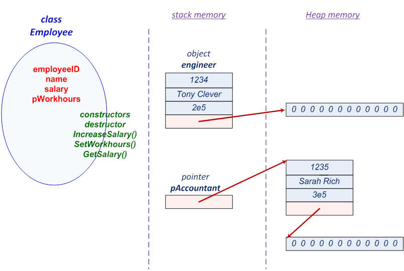
Programmers may also use the pointer this within member functions. This is a good solution to handle ambiguities when the name of a parameter equals with that of a data member:
class Employee{
private:
int employeeID;
string name;
float salary;
public:
Employee(int employeeID=0, string name="", float salary=0){
this->employeeID = employeeID;
this->name = name;
this->salary = salary;
}
};
In normal member functions, the pointer this is declared as Classtype* const this, and in constant member functions as const Classtype*const this.
III.2.2. More about classes
In the previous subchapter, we arrived to classes from structures. We learned how to create well useable classes. Now, it is time to solve tasks with the help of classes.
The present subchapter deals with less general knowledge about classes. This subchapter is mainly dedicated to those who already has some practice in how to create classes.
III.2.2.1. Static class members
In C++, the keyword static can be typed before the data members of classes in order that the objects of these classes could share these members (just like member functions). A static data member that is created in only one instance belongs directly to the class; therefore it is available for it even if there are no objects for that class.
A static data member should not be initialised within its class (independently of its access restriction). An exception to that rule is constituted by data members of type static const integer and enumeration to which a value can be assigned even within the class.
If a static data member is public, then it can be used anywhere in the program code by the name of the class and the scope operator (::). Otherwise, only instances of the class can access these members.
Besides presenting the usage of static members, the following example also demonstrates how to insert constants (static const and enum) in classes. Our mathematics class defined by ourselves (Math) makes it possible for us to call Sin() and Cos() member functions with data in radians or in degrees:
#include <iostream>
#include <iomanip>
#include <cmath>
using namespace std;
class Math {
public:
enum Unit {degree, radian};
private:
static double dDegree2Radian;
static Unit eMode;
public:
static const double Pi;
static double Sin(double x)
{return sin(eMode == radian ? x : dDegree2Radian*x);}
static double Cos(double x)
{return cos(eMode == radian ? x : dDegree2Radian*x);}
static void MeasureUnit(Unit mode = radian) {
eMode = mode; }
void PrintOutPI() { cout.precision(18); cout<<Pi<<endl;}
};
// creating and initialising static members
const double Math::Pi = 3.141592653589793238462;
double Math::dDegree2Radian = Math::Pi/180;
Math::Unit Math::eMode = Math::radian;
As it can be seen in the example, an enumeration can also be placed within a class. The type name Unit and the enumerated constants (degree, radian) can be referenced with a name qualified with the class name. These names have class level scope, independently of the type name preceded by the keyword enum (Math::Unit): Math::radian, Math::degree.
To manage static data members, we use static member functions in general (Math::Sin(), Math::Cos(), Math::MeasureUnit()). However, normal data members cannot be accessed from static functions since the pointer this does not figure among their parameters. The static members of a class can be accessed from non-static member functions without restrictions.
A possible usage of the class Math is presented in the following example:
int main() {
double y = Math::Sin(Math::Pi/6); // counts in radian
Math::MeasureUnit(Math::degree); // counts in degrees
y = Math::Sin(30);
Math::MeasureUnit(Math::radian); // counts in radian
y = Math::Sin(Math::Pi/6);
Math m; // class instance
m.MeasureUnit(Math::degree); // or
m.MeasureUnit(m.degree);
y = m.Sin(30);
m.MeasureUnit(m.radian); // or
m.MeasureUnit(Math::radian);
y = m.Sin(Math::Pi/6);
m.PrintOutPI();
}
III.2.2.2. How to structure classes
The rules of C++ make it possible to structure classes in many ways. In the following examples, each of these methods is strictly separated but in the everyday practice we use them in different combinations.
III.2.2.2.1. Implicit inline member functions
In the first subchapter, the whole definition of member functions is placed in the description of a class. Compilers consider these member functions automatically as inline functions. A big advantage of the solution is that the whole class can be stored in a header file, and the members of the class are logically grouped together. In general, this solution is useful for small-sized classes.
As an example, let's see the class Point, which is able to handle points in the plane.
class Point {
private:
int x,y;
public:
Point(int a = 0, int b = 0) { x = a; y = b; }
int GetX() const { return x; }
int GetY() const { return y; }
void SetX(int a) { x = a; }
void SetY(int a) { y = a; }
void Move(int a, int b) { x = a; y = b; }
void Move(const Point& p) { x = p.x; y = p.y; }
void PrintOut() const { cout<<"("<<x<<","<<y<<")\n"; }
};
III.2.2.2.2. Class structures in C++/CLI applications
The .NET project of Visual C++, Java and C# languages follow principles similar to those above. But there is a big difference: class members are not grouped on the basis of their accessibility, so the accessibility can be provided to each member separately.
class Point {
private: int x,y;
public: Point(int a = 0, int b = 0) { x = a; y = b; }
public: int GetX() const { return x; }
public: int GetY() const { return y; }
public: void SetX(int a) { x = a; }
public: void SetY(int a) { y = a; }
public: void Move(int a, int b) { x = a; y = b; }
public: void Move(const Point& p) { x = p.x; y = p.y; }
public: void PrintOut() const { cout<<"("<<x<<","<<y<<")\n"; }
};
III.2.2.2.3. Storing member functions in separate modules
It is easier to manage a bigger-sized class if its member functions are stored in a separate C++ module. Then the declaration of the class contains not only data members but also the prototype of member functions. The header file containing the description (.H) and the module storing the definition of member functions (.CPP) have the same name in general and refer to their corresponding class.
The description of the class Point in the Point.h header file:
#ifndef __PONT_H__
#define __PONT_H__
class Point {
private:
int x,y;
public:
Point(int a = 0, int b = 0);
int GetX() const;
int GetY() const;
void SetX(int a);
void SetY(int a);
void Move(int a, int b);
void Move(const Point& p);
void PrintOut() const;
};
#endif
The name of member functions has to be qualified with the name of the class (::) in the file Point.cpp:
#include <iostream>
using namespace std;
#include "Point.h"
Point::Point(int a, int b) {
x = a; y = b;
}
int Point::GetX() const {
return x;
}
int Point::GetY() const {
return y;
}
void Point::SetX(int a) {
x = a;
}
void Point::SetY(int a) {
y = a;
}
void Point::Move(int a, int b) {
x = a; y = b;
}
void Point::Move(const Pont& p) {
x = p.x; y = p.y;
}
void Point::PrintOut() const {
cout<<"("<<x<<","<<y<<")\n";
}
Of course, the keyword inline can be used explicitly for member functions; however, in that case, the definition of inline member functions has to be moved from the C++ module to the header file:
#ifndef __PONT_H__
#define __PONT_H__
class Point {
private:
int x,y;
public:
Point(int a = 0, int b = 0);
int GetX() const;
int GetY() const;
void SetX(int a);
void SetY(int a);
void Move(int a, int b);
void Move(const Point& p);
inline void PrintOut() const;
};
void Point::PrintOut() const {
cout<<"("<<x<<","<<y<<")\n";
}
#endif
III.2.2.3. Friend functions and classes
There are cases where the data hiding principles of C++ prevents us to write an efficient program code. However, the friend mechanism makes it possible for us to access the private and protected members of a class from a function outside the class.
A friend declaration can be placed anywhere within the description of that class. An external function, a member function of another class and even a whole other class (that is all of its member functions) can be a "friend". Accordingly, a friend declaration consists of the prototype of the functions and the name of the class, the whole introduced by the keyword class.
It should be noted that a "friend" relationship is not mutual in the case of a friend class because it is only the member functions of the class figuring in the friend declaration that have full access to the members of the class containing that description.
In the following example, the external function Sum(), the public member function named Count() of BClass as well as all data functions of AClass have full access to all members of CClass:
class AClass;
class BClass {
public:
int Count(int x) { return x++; }
};
class CClass {
friend long Sum(int a, int b);
friend int BClass::Count(int x);
friend class AClass;
// ...
};
long Sum(int a, int b) {
return long(a) + b;
}
For another example, let's see the simplified version of our class Point. Since the operation calculating the distance of points cannot be related to any points, a separate external function is written in order that the distance could be determined. The two points are passed as arguments to that function. In order that data members be quickly accessed, a direct access is needed, and this can be realised by the "friend" mechanism.
#include <iostream>
#include <cmath>
using namespace std;
class Point {
friend double Distance(const Point & p1,
const Point & p2);
private:
int x,y;
public:
Point(int a = 0, int b = 0) { x = a; y = b; }
int GetX() const { return x; }
int GetY() const { return y; }
void SetX(int a) { x = a; }
void SetY(int a) { y = a; }
void Move(int a, int b) { x = a; y = b; }
void Move(const Point& p) { x = p.x; y = p.y; }
void PrintOut() const { cout<<"("<<x<<","<<y<<")\n"; }
};
double Distance(const Point & p1, const Point & p2) {
return sqrt(pow(p1.x-p2.x,2.0)+pow(p1.y-p2.y,2.0));
}
int main() {
Point p, q;
p.Move(1,2);
q.Move(4,6);
cout<<Distance(p,q)<<endl;
}
III.2.2.4. What can we also add to classes?
Until now, we have only placed data and functions in classes. We have also added static constants and the type enum to classes.
In the following parts, we will see how to put constants and references in classes, and after that we will also summarise the rules of using nested classes.
III.2.2.4.1. Constant data members of objects
There are cases where a unique constant value is needed to be assigned to object instances, for example a name or an identifier. It is possible if the the data member is preceded by the keyword const and if it is added to the member initialisation list of constructors.
In the following example, objects of type User are created and the public name of users are used as constants:
class User {
string password;
public:
const string name;
User(string user, string psw="") : name(user) {
password=psw;
}
void SetPassword(string newpsw) { password = newpsw;}
};
int main() {
User nata("Lafenita");
User gardener("Liza");
nata.SetPassword("Atinefal1223");
gardener.SetPassword("Azil729");
cout<<nata.name<<endl;
cout<<gardener.name<<endl;
User alias = nata;
// alias = gardener; // error!
}
It should be noted that the traditional member by member copy does not work between objects of the same type if these contain constant members.
III.2.2.4.2. Reference type data members
Since a reference can only be created for an already existing variable, the same is true for references like for constants when objects are constructed. In the following example, the sensor object is linked with the controller object by a reference:
class Sensor {
private:
int data;
public:
Sensor(int x) { data = x; }
int Read() { return data; }
};
class Controller {
private:
Sensor& sensor;
public:
Controller(Sensor& s) : sensor(s) {}
void ReceiveData() { cout<<sensor.Read(); }
};
int main() {
Sensor speed(0x17);
Controller ABS(speed);
ABS.ReceiveData();
}
III.2.2.4.3. Data members as objects
It is frequent to place the object instance of a class in another class as a data member. It is an important rule that when objects of a class like this are created, the inner objects also have to be initialised, which can be achieved by adding them to the member initialisation list of the appropriate constructor call.
Calling a constructor is not necessary if the class of the member object has a constructor without a parameter (default constructor), which is automatically called.
The previous controller-sensor example code can be modified in order that the sensor appear as an object in the controller object:
class Sensor {
private:
int data;
public:
Sensor(int x) { data = x; }
int Read() { return data; }
};
class Controller {
private:
Sensor sensor;
public:
Controller() : sensor(0x17) {}
void ReceiveData() { cout<<sensor.Read(); }
};
int main() {
Controller ABS;
ABS.ReceiveData();
}
III.2.2.5. Pointers to class members
In C++, a pointer to a function cannot be assigned the address of a member function even if their type and parameter list are completely the same. The reason for that is that (non-static) member functions have their effects on the instances of their class. This is also true for the pointers to data members. (Another important difference between these pointers and traditional ones is that the later detailed polymorphism also has its effect if virtual member functions are called with pointers.)
In order to define pointers correctly, we have to use the name of the class and the scope operator:
|
|
forward class declaration, |
|
|
p is a pointer to a data member of type int, |
|
|
pfunct may point to a member function that is called with an argument of type int and that returns no value. |
In the following example, we present how to use pointers to class members. We will access both class members by pointers. If such pointers are used, the members are referenced by the operators .* (dot asterisk) and ->* (arrow asterisk) instead of traditional operators. In order that the address of data members and member functions could be obtained, the "address of" operator (&) has to be used.
#include <iostream>
using namespace std;
class Class {
public:
int a;
void f(int b) { a += b;}
};
int main() {
// pointer to a data member of Class of type int
int Class::*intptr = &Class::a;
// pointer to the member function of Class
// of type void and with a parameter of type int
void (Class::* functptr)(int) = &Class::f;
// creating object instances
Class object;
Class * pobject = new Class();
// accessing the data member with a pointer
object.*intptr = 10;
pobject->*intptr = 100;
// calling the member function f() with a pointer
(object.*functptr)(20);
(pobject->*functptr)(200);
cout << object.a << endl; // 30
cout << pobject->a << endl; // 300
delete pobject;
}
By using typedef, expressions containing pointers are easier to be handled:
typedef int Class::*pointer_int; typedef void (Class::*pointer_funct)(int); … pointer_int intptr = &Class::a; pointer_funct functptr = &Class::f;
III.2.3. Operator overloading
So far, operations belonging to a class have been realised in the form of member functions. And doing operations has meant calling member functions. Program codes become more legible if an operator of a similar content can be used instead of calling functions.
C++ offers the possibility to link a function created by a programmer to a traditional operator, extending the functioning of that operator. This function is called automatically if an operator is used in a specific context.
However, an operator function can be used if one of its parameters is a class of type class or struct. This means that functions without parameters and functions using only arguments of a basic data type cannot become operator functions. General declaration of operator functions:
type operator op(parameterlist);
where the sequence op can be replaced by any of the following operators:
|
[] |
() |
. |
-> |
++ |
-- |
& |
new |
|
* |
+ |
- |
~ |
! |
/ |
% |
new[] |
|
<< |
>> |
< |
> |
<= |
>= |
== |
delete |
|
!= |
^ |
| |
&& |
|| |
= |
*= |
delete[] |
|
/= |
%= |
+= |
-= |
<<= |
>>= |
&= | |
|
^= |
|= |
, |
->* |
After type conversion, an operator function will have the following form:
operator type();
The following operators cannot be overloaded : member selection (.), indirect member selection (.*), scope (::), conditional (?:) and the operators sizeof and typeid since their overloading would result in undesired side effects.
The assignment (=), the "address of" (&) and the comma (,) operations can be applied to objects without overloading.
It should be noted that overloading operators does not result in modifying the operator precedence and associativity, and it is not possible to introduce new operations.
III.2.3.1. Creating operator functions
The choice of an operator function, which realise operator overloading, depends largely on the chosen operator. The following table summarises the possibilities. The type and return value of most operator functions can be provided without restrictions.
|
Expression |
Operator( ♣ ) |
Member function |
External function |
|---|---|---|---|
|
♣a |
+ - * & ! ~ ++ -- |
|
|
|
a♣ |
++ -- |
|
|
|
a♣b |
+ - * / % ^ & | < > == != <= >= << >> && || , |
|
|
|
a♣b |
= += -= *= /= %= ^= &= |= <<= >>= [] |
|
- |
|
a(b, c...) |
() |
|
- |
|
a->b |
-> |
|
- |
Operator functions are generally defined within classes in order that the features of user-defined types could be extended. The operators =, (), [] and -> can only be overloaded by non-static member functions. The operators new and delete are overloaded with static member functions. All other operator functions can be created as member functions or external (in general friend) functions.
The table above summarise well the things we have just said because it categorises into groups the overloadable operations of C++ while leaving out operators of dynamic memory management. The character ♣ in the table replaces the operator, whereas a, b and c are the objects of a class A, B and C.
Most of the overloadable C++ operators can be divided into two categories on the basis of the number of their operands. The following table summarises how to call these two types of operator functions.
Binary operands:
|
Realisation |
Syntax |
Actual call |
|---|---|---|
|
member function |
|
|
|
external function |
|
|
Unary operands:
|
Realisation |
Syntax |
Actual call |
|---|---|---|
|
member function |
|
|
|
member function |
|
|
|
external function |
|
|
|
external function |
|
|
When certain operations are redefined, there are other things that have to be considered than in general. These operators are treated more in the following parts of this chapter.
As an example, let's have a look at the class Vector in which the indexing ([]), value assignment (=) and addition (+, +=) operators are overloaded. The reason for modifying the value assignment operator is to be able to copy better the elements of an array. The operator + is realised by a friend function since the resulting vector does not belong to any of the operands logically. On the contrary, overloading the operation += is carried out by a member function since the elements of the left side operand are modified. The whole declaration of the class (together with inline functions) is contained by the file Vector.h.
#ifndef __VectorH__
#define __VectorH__
class Vector {
inline friend Vector operator+ (const Vector& v1,
const Vector& v2);
private:
int size, *p;
public:
// ----- Constructors -----
// initialising a vector of a given size
Vector(int n=10) {
p = new int[size=n];
for (int i = 0; i < size; ++i)
p[i] = 0; // initialising all elements to zero
}
// Initialising by another vector - a copy constructor
Vector(const Vector& v) {
p = new int[size=v.size];
for (int i = 0; i < size; ++i)
p[i] = v.p[i]; // copying all elements
}
// Init.by a traditional vector with n number of elements
Vector(const int a[], int n) {
p = new int[size=n];
for (int i = 0; i < size; ++i)
p[i] = a[i];
}
// ----- Destructor -----
~Vector() {delete[] p; }
// ----- Member function returning the size -----
int GetSize() const { return size; }
// ----- Operator functions -----
int& operator [] (int i) {
// checking whether index is within bounds
if (i < 0 || i > size-1)
throw i;
return p[i];
}
const int& operator [] (int i) const {
return p[i];
}
Vector operator = (const Vector& v) {
delete[] p;
p=new int [size=v.size];
for (int i = 0; i < size; ++i)
p[i] = v.p[i];
return *this;
}
Vector operator += (const Vector& v) {
int m = (size < v.size) ? size: v.size;
for (int i = 0; i < m; ++i)
p[i] += v.p[i];
return *this;
}
};
// ----- External function -----
inline Vector operator+(const Vector& v1, const Vector& v2) {
Vector sum(v1);
sum+=v2;
return sum;
}
#endif
In order that the example program code be more easily understood, we will give now the readers some further remarks.
Two operator functions were created for the operation of indexing, compilers use the second one with constant vectors. The two operator[]() functions are the overloaded versions of each other although their parameter list is the same. This is possible because C++ compilers also store whether the function is of type const or not in the trace of the function.
The pointer this points to an object; however, the expression *this designates the object itself. Functions of type Vector that return a *this value actually return the actual copy of the object. (It should be noted that functions of type Vektor& return a reference to the actual object because of the statement return *this;)
The usage of the class Vector is exemplified by the following code:
#include <iostream>
using namespace std;
#include "Vector.h"
void show(const Vector& v) {
for (int i=0; i<v.GetSize(); i++)
cout<<v[i]<<'\t';
cout<<endl;
}
int main() {
int a[5]={7, 12}, b[7]={2, 7, 12, 23, 29};
Vector x(a,5); // x: 7 12 0 0 0
Vector y(b,7); // y: 2 7 12 23 29 0 0
Vector z; // z: 0 0 0 0 0 0 0 0 0 0
try {
x = y; // x: 2 7 12 23 29 0 0
x = Vector(a,5);// x: 7 12 0 0 0
x += y; // x: 9 19 12 23 29
z = x + y; // z: 11 26 24 46 58
z[0] = 102;
show(z); // z:102 26 24 46 58
}
catch (int n) {
cout<<"Not a valid array index: "<<n<<endl;
}
const Vector v(z);
show(v); // v:102 26 24 46 58
// v[0] = v[1]+5; // error: assignment of read-only…
}
III.2.3.2. Using type conversion operator functions
C++ language supports that classes could be assigned type conversion. The declaration of a user-defined operator function doing type conversion:
operator type();
The type of the return value of the function equals with the type figuring in the name of the function. The type conversion operator function can only be a function without return value and argument list.
In the following example, the type Complex is realised as a class. The only constructor in the example not having an argument of type Complex converts a double into a Complex. For the opposite conversion, we create a conversion operator named double.
#include <cmath>
#include <iostream>
using namespace std;
class Complex {
public:
Complex () { re=im=0; }
Complex(double a) : re(a), im(0) { }
// conversion constructor
Complex(double a, double b) : re(a), im(b) { }
// conversion operator
operator double() {return sqrt(re*re+im*im);}
Complex operator *= (const Complex & k) {
Complex t;
t.re=(k.re*re)-(k.im*im);
t.im=(k.re*im)+(re*k.im);
return *this = t;
}
void Print() const { cout << re << "+" << im << "i"; }
private:
double re, im;
friend Complex operator*(const Complex&, const Complex&);
};
Complex operator*(const Complex& k1, const Complex& k2) {
Complex k=k1;
k*= k2;
return k;
}
int main() {
Complex k1(7), k2(3,4), k3(k2);
cout << double(k3)<< endl; // printed value: 5
cout <<double(Complex(10))<< endl; // printed value: 10
Complex x(2,-1), y(3,4);
x*=y;
x.Print(); // 10+5i
}
It should be noted that three constructors of the class Complex can be replaced by one if default arguments are used:
Complex(double a=0, double b=0) : re(a), im(b) {}
III.2.3.3. Extending classes with input/output operations
C++ makes it possible for us to "teach" I/O data streams based on classes to handle the objects of user-defined classes. From among the data stream classes, istream is responsible for data input, whereas ostream for data output.
In order to carry out input/output operations, we use the overloaded versions of the operators >> and <<. In order to achieve the desired functioning, we should write our proper versions of the above mentioned operations as friend operator functions, as it can be seen in the extended version of the class Complex:
#include <cmath>
#include <sstream>
#include <iostream>
using namespace std;
class Complex {
public:
Complex(double a=0, double b=0) : re(a), im(b) {}
operator double() {return sqrt(re*re+im*im);}
Complex operator *= (const Complex & k) {
Complex t;
t.re=(k.re*re)-(k.im*im);
t.im=(k.re*im)+(re*k.im);
return *this = t;
}
private:
double re, im;
friend Complex operator*(const Complex&, const Complex&);
friend istream & operator>>(istream &, Complex &);
friend ostream & operator<<(ostream &, const Complex &);
};
Complex operator*(const Complex& k1, const Complex& k2) {
Complex k=k1;
k*= k2;
return k;
}
// The format of data input: 12.23+7.29i and 12.23-7.29i
istream & operator>>(istream & is, Complex & c) {
string s;
getline(is, s);
stringstream ss(s);
if (!(ss>>c.re>>c.im))
c=Complex(0);
return is;
}
// The format of data output: 12.23+7.29i and 12.23-7.29i
ostream & operator<<(ostream & os, const Complex & c) {
os<<c.re<<(c.im<0? '-' : '+')<<fabs(c.im)<<'i';
return os;
}
int main() {
Complex a, b;
cout<<"Please enter a complex number: "; cin >> a;
cout<<"Please enter a complex number: "; cin >> b;
cout<<"The product of the complex numbers: " << a*b;
cout<<endl;
}
III.3. Inheritance (derivation)
The previous sections treated how tasks can be solved with classes independent from one another. However, object-oriented programming offers more features besides that. When a problem is processed in an object-oriented manner, the program developing method named derivation (inheritance) is often applied. Derivation makes it possible to use the data and operations of already existing classes in a new aspect or to use or expand them in compliance with the need of the new task. Consequently, problems are not solved with the help of one (big) class but with the help of a system (generally a hierarchy) of classes.
Inheritance is the most important feature of object-oriented C++. This mechanism makes it possible to create (to derive) new classes from already existing ones. Derivation means that a new class inherits the public and protected properties (data members) and behaviour (member functions) of already existing classes and it then uses them as its own. However, already existing classes may be extended with a new class, new data members and member functions may be defined or inherited member functions may be reinterpreted (replaced) if they become deprecated concerning their functioning (polymorphism).
Specialised literature uses many expressions to designate the notions related to inheritance. First, we will recapitulate these expressions and underline those that are used in C++.
|
|
class A, that is derived or from which members are inherited: base class , ancestor class , parent class, superclass the operation: inheritance , derivation , extending, subclassing class B, the result of derivation: descendant class , derived class , extended class, child class, subclass |
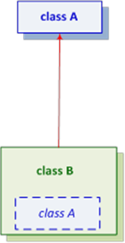
The C++ program code that realises the relation above:
class ClassA {
// ...
};
class ClassB : public ClassA {
// ...
};
Specialised literature does not use notions consequently: for example, the notions 'base class' or 'ancestor class' of a given class may designate any ancestor and the notions 'descendant class' or 'derived class' may be used to designate any class created by derivation. The present book uses these notions to designate direct ancestor and direct descendant classes, respectively.
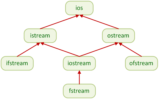
C++ supports multiple inheritance, during which a new class is derived from more base classes (that is it has more direct ancestors) (Figure III.5, “The multiple inheritance of I/O classes in C++”). The class structure that results from multiple inheritance has a mesh structure which is difficult to manage and to interpret. That is why, this solution is only used at a restricted extent. So it is often replaced with single inheritance. The latter means that a class may have at most one ancestor class and any number of descendants. Multi-level inheritance results in a real tree structure (class hierarchy) (Figure III.6, “Hierarchy of geometrical classes”).
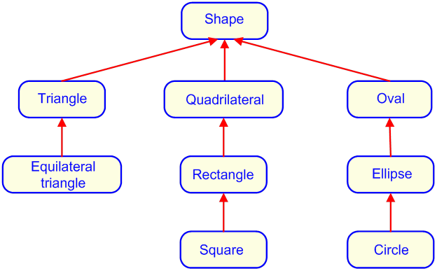
III.3.1. Derivation of classes
A derived (descendant) class is a class that inherits its data members and member functions from one or more already defined class(es). The class from which a derived class inherits is called base class (ancestor class). A derived class may also become a base class for other classes, so it can contribute to a class hierarchy.
A derived class inherits all the members of its base class; however, it only have access to the public and protected members of its base class as its own. The protected access involves a double behaviour. It means private access to the users of the given class, who create objects from that; however, it offers public access to developers who derive new classes from it. In general, member functions are defined to be public or protected while data members are protected or private. (Private access hides these members even from the member functions of their derived classes.) Derived classes may complete inherited members with new data members and member functions.
The place where a derivation is indicated in a program code is the class header where the mode of derivation (public, protected, private) is indicated before the names of base classes:
class Derived : public Base1, ...private BaseN
{
// the class body
};
Independently of their access restriction in their base class, constructors, destructors, assignment operator and friend relations are not inherited. In most cases, it is public inheritance that is used because, in this way, descendant objects can replace their ancestor objects in all contexts.
The following example shows how to use inheritance by defining points in a two-dimensional plane and in a three-dimensional space. The resulting class hierarchy is very simple (the red arrow points directly to the direct base class):
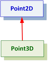
class Point2D {
protected:
int x,y;
public:
Point2D(int a = 0, int b = 0) { x = a; y = b; }
void GetPoint2D(int& a, int& b) const { a=x; b=y;}
void Move(int a=0, int b=0) { x = a; y = b; }
void Move(const Point2D& p) { x = p.x; y = p.y; }
void PrintOut() const {
cout<<'('<<x<<','<<y<<')'<<endl; }
}
class Point3D : public Point2D {
protected:
int z;
public:
Point3D(int a=0, int b=0, int c=0):Point2D(a,b),z(c) {}
Point3D(Point3D & p):Point2D(p.x, p.y),z(p.z) {}
void GetPoint3D(int& a, int& b, int& c) const {
a = x; b = y; c = z; }
void Move(int a=0, int b=0, int c=0) {
x = a; y = b; z = c; }
void Move(const Point3D& p) {
Point2D::x = p.x; y = p.y; z = p.z;}
void PrintOut() const {
cout<<'('<<x<<','<<y<<','<<z<<')'<<endl;}
};
void Visualise(const Point2D & p) {
p.PrintOut();
}
int main() {
Point2D p1(12,23), p2(p1), p3;
Point3D q1(7,29,80), q2(q1), q3;
p1.PrintOut(); // (12,23)
q1.PrintOut(); // (7,29,80)
// q1 = p1; // ↯ - error!
q2.Move(10,2,4);
p2 = q2;
p2.PrintOut(); // (10,2)
q2.PrintOut(); // (10,2,4)
q2.Point2D::PrintOut(); // (10,2)
Visualise(p2); // (10,2)
Visualise(q2); // (10,2)
}
In the example, elements that are marked with blue are program elements used as a consequence of inheritance. These elements are treated later in this chapter.
It can be seen that the objects of the class created by public derivation replace the object of the base class in all cases (assignment, function argument, ...):
p2 = q2; Visualise(q2);
The reason for that is that a derived class completely comprises its base class in case of inheritance. However, this is not true in the opposite direction, so the following value assignment leads to a compilation error:
q1 = p1; // ↯
The keywords public, protected and private used in a derivation list restrict the access of inherited (public and protected) members in their new classes, in the way summarised in the following table:
|
Mode of inheritance |
Access in the base class |
Access in the derived class |
|---|---|---|
|
public |
public protected |
public protected |
|
protected |
public protected |
protected protected |
|
private |
public protected |
private private |
When a class is derived as public, the inherited members keep their access mode in their base class, whereas if a derivation is private, the inherited members become the private members in the derived class, therefore they become hidden to the users of the new class and to developers who would develop it further. If a class is derived as protected, the inherited members become protected in the new class so they can be further inherited. (The default derivation mode for base classes of type class is private, whereas for those of type struct, it is public.)
This default behaviour leads to an appropriate result in most cases and offers an appropriate access to the inherited members of derived classes. However, the access of any member (the access type of which is protected or public in the base class) can be manually set directly, too. For that purpose, the name of the members qualified with the base class has to be simply inserted in the appropriate access type group. It should be made sure that a new access type cannot give members an access superior to that in their base class. For example, if a member that is protected in the ancestor class is inherited privately, it automatically becomes private in the derived class, but it can be placed in the protected access group (but not in the public group).
To exemplify this, let's derive by private derivation the class named Point3D but let's assign the data members the same access restriction as the one they had if the derivation was public.
class Point3D : private Point2D {
protected:
int z;
Point2D::x;
Point2D::y;
public:
Point3D(int a=0, int b=0, int c=0):Point2D(a,b),z(c) {}
Point3D(Point3D & p):Point2D(p.x, p.y),z(p.z) {}
void GetPoint3D(int& a, int& b, int& c) const {
a = x; b = y; c = z; }
void Move(int a=0, int b=0, int c=0) {
x = a; y = b; z = c; }
void Move(const Point3D& p) {
x = p.x; y = p.y; z = p.z;}
void PrintOut() const {
cout<<'('<<x<<','<<y<<','<<z<<')'<<endl;}
Point2D:: GetPoint2D;
};
III.3.2. Initialising base class(es)
In order that base class(es) be initialised, it is the extended version of member initialisation lists that is used, where, besides members, the constructor calls of direct ancestors are also enumerated.
class Point3D : public Point2D {
protected:
int z;
public:
Point3D(int a=0, int b=0, int c=0):Point2D(a,b),z(c) {}
Point3D(Point3D & p):Point2D(p.x, p.y),z(p.z) {}
// …
};
When a derived class is instantiated, the compiler calls the constructors in the following order:
The constructors of the base class are executed in the order corresponding to the initialisation list.
The constructors of the member objects of the derived class are called in the order in which object members were defined (they do not figure in this example).
The constructor of the derived class is executed.
Calling the constructor of the ancestor class is not necessary, if the base class has a constructor without parameters, which is called automatically by compilers. Since this condition is fulfilled in this example, the second constructor can be realised in the following form:
Point3D(Point3D & p) { *this = p;}
(Another condition of that solution is public inheritance, which is also fulfilled.)
When a class hierarchy is developed, it is enough that each class takes care of initialising only its direct ancestor(s). In that way, all parts of the instance of classes that are situated at a higher level (farer from the root) are automatically assigned an initial value if the object is created.
When the derived object instance is destroying, destructors are executed in the order that is reverse to the above described one.
The destructor of the derived class is executed.
The destructors of the member objects of the derived class are called in the order reverse to their definition.
The destructors of base classes are executed, in an order opposite to that of the classes in the derivation list.
III.3.3. Accessing class members in case of inheritance
In Section III.2, “Classes and objects” class members were divided into two groups on the basis of their access: accessible and inaccessible. These two groups are further nuanced by inherited and not inherited categories. Section III.3.1, “Derivation of classes” that detailed the way of deriving classes, described how basic access restrictions work. Now we will only give an overview of further solutions that precise what we have already learnt about inheritance.
III.3.3.1. Accessing inherited members
In general, the inherited members of derived classes can be accessed in the same way as their own members. However, if a data member or a member function is created with the same name in the derived class as the name of an inherited member, then the member of the ancestor class becomes hidden. In such cases, the scope operator has to be used to reference them:
Class_name::member_name
Compilers identify member names together with their class scope, that is why all member names can be used in the form above. The example code of Section III.3.1, “Derivation of classes” shows us some examples for the things that has been said.
class Point3D : public Point2D {
protected:
int z;
public:
Point3D(int a=0, int b=0, int c=0):Point2D(a,b),z(c) {}
Point3D(Point3D & p):Point2D(p.x, p.y),z(p.z) {}
// …
void Move(const Point3D& p) {
Point2D::x = p.x; y = p.y; z = p.z;}
// …
};
int main() {
Point2D p1(12,23), p2(p1), p3;
Point3D q1(7,29,80), q2(q1), q3;
q2.Point2D::PrintOut();
q2.Point2D::Move(1,2); // Moving in the x-y plane
q2.Point2D::Move(p1);
// …
}
The following table summarises what kind of members the classes of the example code have access. If a member is hidden, it is provided with their class name:
|
The members of the base class Point2D: |
The members of the derived class Point3D |
|---|---|
|
|
|
III.3.3.2. The friend relationship in inheritance
In a derived class, a friend of the base class can only access the members inherited from the base class. A "friend" of a derived class can only access public and protected members from the base class.
III.3.4. Virtual base classes in case of multiple inheritance
In case of multiple inheritance, it may be a problem if the same base class appears as many instances in the derived class. If virtual base classes are used, problems of that type can be avoided (Figure III.7, “Using virtual base classes”).
class Base {
int q;
public:
Base(int v=0) : q(v) {};
int GetQ() { return q;}
void SetQ(int q) { this->q = q;}
};
// the virtual base class named Base
class Base1 : virtual public Base {
int x;
public:
Base1(int i): x(i) {}
};
// the virtual base class named Base
class Base2: public virtual Base {
int y;
public:
Base2(int i): y(i) {}
};
class Descendant: public Base1, public Base2 {
int a,b;
public:
Descendant(int i=0,int j=0): Base1(i+j),Base2(j*i),a(i),b(j) {}
};
int main() {
Descendant descendant;
descendant.Base1::SetQ(100);
cout << descendant.GetQ()<<endl; // 100
cout << descendant.Base1::GetQ()<<endl; // 100
cout << descendant.Base2::GetQ()<<endl; // 100
descendant.Base1::SetQ(200);
cout << descendant.GetQ()<<endl; // 200
cout << descendant.Base1::GetQ()<<endl; // 200
cout << descendant.Base2::GetQ()<<endl; // 200
}
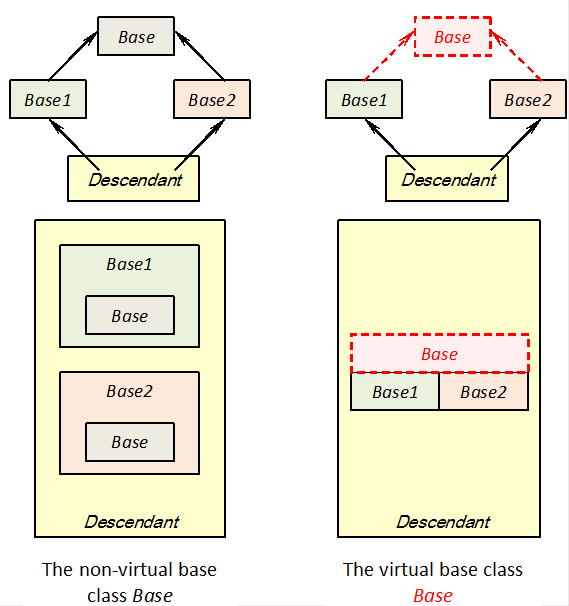
A virtual base class will only be present in only one instance in its derived classes, independently of its number of occurrences in the inheritance chain. In the example, the data member named q of the virtual base class are inherited both by the base classes Base1 and Base2. Because of its virtuality, the class named Base occurs only in one instance, so Base1::q and Base2::q reference the same data member. Without using the keyword virtual, Base1::q and Base2::q designate different data members, which leads to a compilation error, since the compiler will not know for sure how to resolve the reference descendant.GetQ().
III.3.5. Inheritance and/or composition?
A big advantage of C++ programming language is that it supports the reusability of program code. Reusing means that a new program code is made without modifying the original one. If the object-oriented tools of C++ are used, there are three approaches to choose from:
The most simple and frequent reuse of a code stored in a given class is when an object instance is created or when already existing objects ( cin , cout , string , STL etc.) are used in a program.
class X {
// …
};
int main() {
X a, *pb;
pb = new X();
cout<<"C++"<<endl;
// …
delete pb;
}
Another possibility is to place objects of other classes in our own codes as member objects. Since the new class is created by reusing already existing ones, this method is called composition. During composition, the relation between new and included objects becomes a (has-a) relation. If the new object will only contain a pointer or a reference to other objects, it is called an aggregation.
class X {
// …
};
class Y {
X x; // composition
};
class Z {
X& x; // aggregation
X *px;
};
The third solution is related to the subject of the present chapter. When a new class is created by public derivation from other classes, then the relationship is of an is-a type. This relation means that a derived object behaves exactly the same way as its ancestor class (that is the derived object is also an ancestor object); however, this is not true in the reverse direction.
// base class
class X {
// …
};
// derived class
class Y : public X {
// …
};
If a problem is solved in an object-oriented way, it has to be determined that the desired model is achieved better by inheritance or by composition. The decision is not easy to take but the following guidelines may help a lot:
The starting point should be composition. However, if later it turns out that a class is actually a special type of another class, inheritance should be used.
Derivation is really needed if there is a need to cast the type of a derived class to the base class. For example, if all elements of a geometrical system is to be stored in a linked list.
The starting point should be composition. However, if later it turns out that a class is actually a special type of another class, inheritance should be used.
The following two example codes clearly show the differences and similarities between composition and derivation. In both cases, it is the class Point that is reused. This class is stored in the file named Point.h.
#ifndef __POINT_H__
#define __POINT_H__
class Point {
protected:
int x,y;
public:
Point(int a = 0, int b = 0) : x(a), y(b) {}
Point(const Point& p) : x(p.x), y(p.y) {}
int GetX() const { return x; }
int GetY() const { return y; }
void SetX(int a) { x = a; }
void SetY(int a) { y = a; }
void Move(int a, int b) { x = a; y = b; }
void Move(const Point& p) { x = p.x; y = p.y; }
void PrintOut() const { cout<<'('<<x<<','<<y<<')'<< endl; }
};
#endif
III.3.5.1. Reuse with composition
In real life, complex objects are often made up of smaller and simpler objects. For example, a car can be put together from a chassis, an engine, some tyres, a gear box, steerable wheels and a huge quantity of other spare parts. If the composition is done, the car has-a gearbox, has an engine, etc.
In the example named Circle, the circle has a centre which is stored in a member object of type Point named p. It should be noted that only the public members of the class Point can be accessed from the member functions of the class Circle.
#include "Point.h"
class Circle {
protected:
int r;
public:
Point p; // composition
Circle(int x=0, int y=0, int r=0)
: p(x, y), r(r) {}
Circle(const Point& p, int r=0)
: p(p), r(r) {}
int GetR() {return r;}
void SetR(int a) { r = a; }
};
int main() {
Circle c1(100, 200, 10);
c1.p.PrintOut();
cout<<c1.p.GetX()<<endl;
cout<<c1.GetR()<<endl;
}
III.3.5.2. Reuse by public inheritance
Like for composition, there are many examples in real life for inheritance. Everyone inherits genes from his/her parents; C++ language has also inherited many things from C language, which also inherited one part of its properties of its ancestors. In inheritance, the attributes and behaviour of base class(es) are obtained directly, and they may be extended or precised.
In our example, the object of type Point as the centre of the circle becomes integrated in the object of type Circle, which completely complies with the definition of a circle. Contrary to composition, the protected and public members of the class Point can be accessed from the member functions of the class Circle.
#include "Point.h"
class Circle : public Point { // inheritance
protected:
int r;
public:
Circle(int x=0, int y=0, int r=0)
: Point(x, y), r(r) {}
Circle(const Point & p, int r=0)
: Point(p), r(r) {}
int GetR() {return r;}
void SetR(int a) { r = a; }
};
int main() {
Circle c1(100, 200, 10);
c1.PrintOut();
cout<<c1.GetX()<<endl;
cout<<c1.GetR()<<endl;
}
III.4. Polymorphism
In C++, polymorphism rather means that the object of a derived class is accessed by a pointer or a reference in the base class. Although the subject of this subsection is the solution called subtype or run-time polymorphism or simply overriding, let's review further "polymorphous" solutions of C++.
Coercion polymorphism means implicit and explicit type casts. In that case, the polymorphism of a given operation is made possible by different types that may be converted if needed.
As an opposite to coercion, the so-called ad-hoc („for that purpose”) polymorphism is better known by the name of function overloading. In that case, a compiler chooses the appropriate function from the variants on the basis of parameter types.
The extended version of this polymorphism is called parametrical or compile-time polymorphism, which makes it possible to execute the same code with any type. In C++, parametric polymorphism is realised by function and class templates. Using templates actually means reusing a C++ source code.
Previously, we have said that a derived class inherits all properties and behaviour (operations) of its ancestor. These inherited member functions can be reused without restrictions in the objects of the derived class since they comprise their ancestors. Since a derived class is often specialised, it may be necessary that certain inherited functions work in another way. This need is satisfied by introducing virtual member functions. Thanks to real-time polymorphism, an object may react to the same message in another way, depending on the level it occupies in the class hierarchy. And the choice of the member function that will be called from the inheritance chain only becomes known during execution (late binding).
III.4.1. Virtual member functions
A virtual function is a public or protected member function of the base class. It can be redefined in the derived class in order that the behaviour of the class would change. A virtual function is generally called by a reference or a pointer of a public base class, the actual value of which is determined at run-time (dynamic binding, late binding).
In order that a member function become virtual, the keyword virtual has to be provided in the class before the declaration of the function:
class Example {
public:
virtual int vf();
};
It is not necessary that a virtual function in the base class have a definition as well. Instead, the prototype of the function should be ended with the expression =0; . In that case, it is a so-called pure virtual function:
class Example {
public:
virtual int pvf() = 0;
};
An object instance cannot be created from a class containing one or more pure virtual functions (an abstract class). An abstract class can only be used as a starting point, as a base class for inheritance.
In case a member function becomes virtual at a level in the class hierarchy, then it can be replaced in any subsequent class in the inheritance chain.
III.4.2. Redefining virtual functions
If a function is declared as virtual in the base class, then it preserves this property during inheritance. In the derived class, a virtual function can be redefined with another version but the inherited version may also be used. If a new version is defined, it is not necessary to use the keyword virtual.
If a derived class inherits a pure virtual function, it has to be redefined by a new version, otherwise the new class will also be abstract. A derived class may contain virtual functions that it has not inherited from its direct base class.
The prototype of a virtual function redefined in the derived class has to be precisely identical (name, type, parameter list) with the one defined in the base class. If the parameterizations of the two declarations are not completely identical, then it is not redefining but overloading.
|
In the following example code, each shape calculates its own area and perimeter; however, visualisation is carried out by an abstract base class (Shape). The hierarchy of class is represented in the following figure: |
|
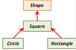
// Abstract base class
class Shape {
protected:
int x, y;
public:
Shape(int x=0, int y=0) : x(x), y(y) {}
virtual double Area()=0;
virtual double Perimeter()=0;
void Visualise() {
cout<<'('<<x<<','<<y<<")\t";
cout<<"\tArea: "<< Area();
cout<<"\tPerimeter: "<< Perimeter() <<endl;
}
};
class Square : public Shape {
protected:
double a;
public:
Square(int x=0, int y=0, double a=0)
: Shape(x,y), a(a) {}
double Area() {return a*a;}
double Perimeter() {return 4*a;}
};
class Rectangle : public Square {
protected:
double b;
public:
Rectangle(int x=0, int y=0, double a=0, double b=0)
: Square(x,y,a), b(b) {}
double Area() {return a*b;}
double Perimeter() {return 2*(a+b);}
};
class Circle : public Square {
const double pi;
public:
Circle(int x=0, int y=0, double r=0)
: Square(x,y,r), pi(3.14159265) {}
double Area() {return a*a*pi;}
double Perimeter() {return 2*a*pi;}
};
int main() {
Square s(12,23,10);
cout<<"Square: ";
s.Visualise();
Circle c(23,12,10);
cout<<"Circle: ";
c.Visualise();
Rectangle r(12,7,10,20);
cout<<"Rectangle: ";
r.Visualise();
Shape* shapes[3] = {&s, &c, &r} ;
for (int i=0; i<3; i++)
shapes[i]->Visualise();
}
Virtual functions and public inheritance make it possible to create external functions that can be called by every object in the class hierarchy:
void VisualiseAll(Shape& a) {
cout<<"Area: "<<a.Area()<<endl;
cout<<"Perimeter: "<<a.Perimeter()<<endl;
}
III.4.3. Early and late binding
In order to explain more how run-time polymorphism works, we will examine, through examples, the resolution of member function calls at compilation time (early binding) and at run-time (late binding).
In the example codes, two member functions having the same prototype are defined (GetName(), GetValue()) both in the base class and the derived class. The main() function contains a pointer and a reference to an instance of the derived class. The pointer (pA) and the reference (rA) are of the type of the base class.
III.4.3.1. Static early binding
During early binding, compilers integrate statically direct member function calls into the code. In the case of classes, this is the default operation mode, which is clearly reflected by the following example code.
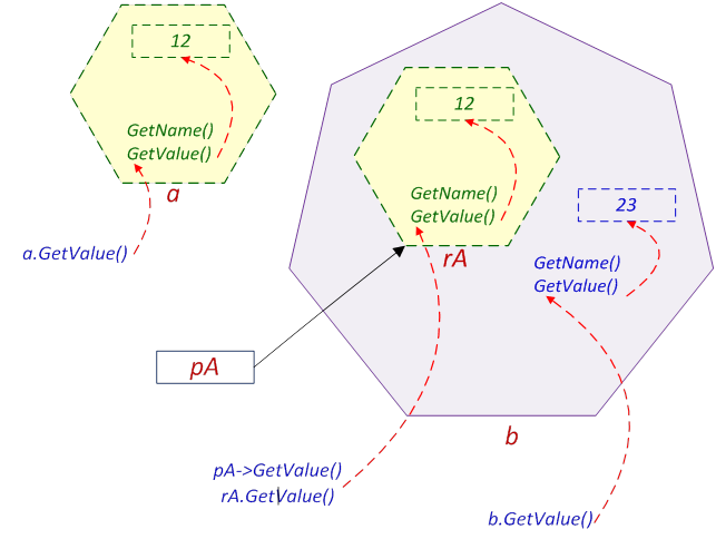
class Base {
protected:
int value;
public:
Base(int a=0) : value(a) { }
const char* GetName() const { return "Base"; }
int GetValue() const { return value; }
};
class Derived: public Base {
protected:
int value;
public:
Derived(int a=0, int b=0) : Base(a), value(b) { }
const char* GetName() const { return "Derived"; }
int GetValue() const { return value; }
};
int main() {
Base a;
Derived b(12, 23);
a = b;
Base &rA = b;
Base *pA = &b;
cout<<"a \t" << a.GetName()<<"\t"<< a.GetValue()<<endl;
cout<<"a \t" << b.GetName()<<"\t"<< b.GetValue()<<endl;
cout<<"rA\t" << rA.GetName()<<"\t"<< rA.GetValue()<<endl;
cout<<"pA\t" << pA->GetName()<<"\t"<< pA->GetValue()<<endl;
}
The calls of the member function GetValue() is presented in Figure III.8, “Early binding example”. The results:
a Base 12 b Derived 23 rA base 12 pA Base 12
III.4.3.2. Dynamic late binding
The situation changes a lot (Figure III.8, “Early binding example”), if the member functions GetName(), GetValue() are made virtual in the class Base.
class Base {
protected:
int value;
public:
Base(int a=0) : value(a) { }
virtual const char* GetName() const { return "Base"; }
virtual int GetValue() const { return value; }
};
The results have also changed:
a Base 12 b Derived 23 rA Derived 23 pA Derived 23

Compilers place the calls of virtual functions indirectly in the code: as jumps to the address stored in the memory. The virtual method table (VMT) used for storing addresses is created for each class during execution, at the first instantiation of the given class. VMT contains the address of redefined virtual functions. Virtual functions having the same name and being situated in the class hierarchy have the same index in these tables, which makes it possible to replace completely virtual member functions.
III.4.3.3. Virtual method table
In case a class has one or more virtual member functions, compilers complete the object with a "virtual pointer" to the global data table called virtual method table (VMT) or virtual function table (VFTable). VMT contains function pointers to the virtual member functions redefined the last of the given class and the base classes (Figure III.10, “Virtual method tables of the example code”). The address of the virtual functions having the same name has the same index in these tables.
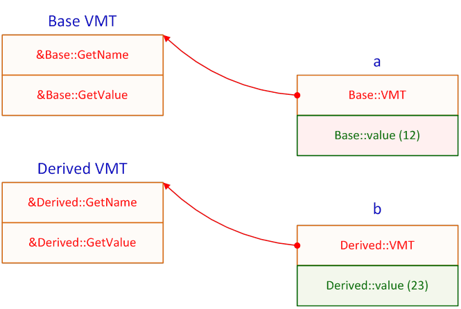
VMTs for classes are created at run-time when the first constructor is called. As a consequence, the relation between the caller and the called member function is also realised at run-time. The compiler will only insert in the code a call that takes place by using the ith element of the VMT (call VMT[i]).
III.4.4. Virtual destructors
A destructor can be defined as a virtual function. If the destructor of the base class is virtual, then the destructor of all classes derived from that will also be virtual. That is why, it is sure that it is always the appropriate destructor that is called if the object ceases to exist even if a pointer or a reference of the type of a base class references that instance of the derived class.
In order to activate this mechanism, it is enough to place a virtual, empty destructor in a class somewhere in the beginning of the inheritance chain:
class Base {
protected:
int value;
public:
Base(int a=0) : value(a) { }
virtual const char* GetName() const { return "Base"; }
virtual int GetValue() const { return value; }
virtual ~Base() {}
};
III.4.5. Abstract classes and interfaces
As we have already seen, abstract classes are good bases for inheritance chains. In C++, there are no keywords to designate abstract classes, they can only be recognised if we know whether they contain pure virtual functions or not. The reason for treating them again in this part is to follow the traditions of other programming languages, and to find elements from them that can be realised in C++ as well.
The Java, C# and Object Pascal programming languages support only single inheritance; however, they make it possible to implement any number of interfaces. In a C++ environment, an interface is an abstract class that only has virtual functions. The only aim of interfaces is to force developers (if they derive them) to create the member functions that have been declared as public in them.
The traps of multiple inheritance can be avoided if the base classes only contain one "real" class (that is a class that has data members, too) and the others are only interface classes. (The names of interfaces classes generally begin with a capital "I".)
To exemplify interfaces, in a previous class named Point, we separate now the class storing the geometrical values and the interface defining the ability to move, since the latter is not always needed.
// the geometrical Point class
class Point {
protected:
int x, y;
public:
Point(int a = 0, int b = 0) : x(a), y(b) {}
Point(const Point& p) : x(p.x), y(p.y) {}
int GetX() const { return x; }
int GetY() const { return y; }
void SetX(int a) { x = a; }
void SetY(int a) { y = a; }
void PrintOut() const { cout<<'('<<x<<','<<y<<')'<< endl; }
};
// an abstract class needed for moving - interface
class IMove {
public:
virtual void Move(int a, int b) = 0;
virtual void Move(const Point& p) = 0;
};
// a Point that is able to move
class MovingPoint: public Point, public IMove {
public:
MovingPoint(int a=0, int b=0) : Point(a,b) {}
void Move(int a, int b) { x = a; y = b; }
void Move(const Point& p) {
x = p.GetX();
y = p.GetY();
}
};
int main() {
Point fixPoint(12, 23);
fixPoint.PrintOut(); // (12, 23)
MovingPoint movingPoint;
movingPoint.PrintOut(); // (0, 0)
movingPoint.Move(fixPoint);
movingPoint.PrintOut(); // (12, 23)
}
III.4.6. Run-time type informations in case of classes
Visual development kits store Run-time Type Information, RTTI for each object instances. With the help of them, it is executing environments that may be entrusted with identifying the type of objects, so new data members do not have to introduced for that purpose.
In order that RTTI mechanism function correctly, a polymorphous base class has to be created, that is at least a virtual member function should be inserted into it and the storage of RTTI has to be enabled. (The possibility to enable this feature can be found among the settings of the compiler.) In order that the type of pointers and references be identified, the operations dynamic_cast and typeid are used. In order that appropriate type cast be carried out, the operator dynamic_cast is used.
The operator typeid returns an object of type const type_info , the members of which provide information about the type of the operand. The character sequence returned by the member function named name() of the object depends on the used compiler. In order to use the operator, the header file typeinfo should be included in the code.
#include <typeinfo>
#include <iostream>
using namespace std;
class Ancestor {
public:
virtual void Vf(){} // without this, RTTI is not stored
void FunctAncestor() {cout<<"Ancestor"<<endl;}
};
class Descendant : public Ancestor {
public:
void FunctDescendant() {cout<<"Descendant"<<endl;}
};
int main() {
Descendant * pDescendant = new Descendant;
Ancestor * pAncestor = pDescendant;
// the type_info of the pointer:
const type_info& tiAncestor = typeid(pAncestor);
cout<< tiAncestor.name() <<endl;
// the type_info of the Descendant:
const type_info& tiDescendant = typeid(*pAncestor);
cout<< tiDescendant.name() <<endl;
// points to the Descendant?
if (typeid(*pAncestor) == typeid(Descendant))
dynamic_cast<Descendant *>(pAncestor)
->FunctDescendant();
// points to the Descendant?
if (dynamic_cast<Descendant*>(pAncestor))
dynamic_cast<Descendant*>(pAncestor)
->FunctDescendant();
delete pDescendant;
}
The following example code needs run-time type information if members of different classes are to be accessed.
#include <iostream>
#include <string>
#include <typeinfo>
using namespace std;
class Animal {
protected:
int legs;
public:
virtual const string Species() = 0;
Animal(int n) {legs=n;}
void Info() {
cout<<"A(n) "<<Species()<<" has "
<<legs<<" leg(s)."<<endl;
}
};
class Fish : public Animal {
protected:
const string Species() {return "fish";}
public:
Fish(int n=0) : Animal(n) {}
void Swims() {cout<<"swims"<<endl;}
};
class Bird : public Animal {
protected:
const string Species() {return "bird";}
public:
Bird(int n=0) : Animal(n) {}
void Flies() {cout<<"flies"<<endl;}
};
class Mammal : public Animal {
protected:
const string Species() {return "mammal";}
public:
Mammal(int n=4) : Animal(n) {}
void Runs() {cout<<"runs"<<endl;}
};
int main() {
const int db=3;
Animal* p[db] = {new Bird, new Fish, new Mammal};
// accessing data without RTTI
for (int i=0; i<db; i++)
p[i]->Info();
// processing with the help of RTTI
for (int i=0; i<db; i++)
if (dynamic_cast<Fish*>(p[i])) // Fish?
dynamic_cast<Fish*>(p[i])->Swims();
else
if (typeid(*p[i])==typeid(Bird)) // Bird?
dynamic_cast<Bird*>(p[i])->Flies();
else
if (typeid(*p[i])==typeid(Mammal)) // Mammal?
dynamic_cast<Mammal*>(p[i])->Runs();
for (int i=0; i<db; i++)
delete p[i];
}
For the sake of comparison, let's also have a look at the version of the code above that does not use run-time type information. In that case, the value of the virtual function Species() of the class Animal can be used to identify the class and type cast is carried out by the operator static_cast. It is only the content of the main() function that has changed:
int main() {
const int db=3;
Animal* p[db] = {new Bird, new Fish, new Mammal};
for (int i=0; i<db; i++)
p[i]->Info();
for (int i=0; i<db; i++)
if (p[i]->Species()=="fish")
static_cast<Fish*>(p[i])->Swims();
else
if (p[i]->Species()=="bird")
static_cast<Bird*>(p[i])->Flies();
else
if (p[i]->Species()=="mammal")
static_cast<Mammal*>(p[i])->Runs();
for (int i=0; i<db; i++)
delete p[i];
}
The results of executing both versions are the same:
A(n) bird has two leg(s). A(n) fish has 0 leg(s). A(n) mammal has 4 leg(s). flies swims runs
III.5. Class templates
The solutions of most typed languages depend on types: when a useful function or class is created, it only works correctly with data of the types fixed in it. If the same function/class is to be used for other types of data, it has to be rewritten by replacing the concerned types.
C++ language introduces function and class templates to prevent developers from doing this kind of type replacing method. The only task of a programmer in C++ is to write the needed function or class and to mark all types to be replaced, and the other things are done by compilers.
III.5.1. A step-be-step tutorial for creating and using class templates
As an introduction, we will review how to make and use templates step by step. For that purpose, we rely on knowledge already treated in the present book.
As an example, let's see the class named IntArray, which is a simplified class handling an one-dimensional integer array of 32 elements with bound index checking.
#include <iostream>
#include <cassert>
#include <cstring>
using namespace std;
class IntArray {
public:
IntArray(bool initialise = true) : size(32) {
if (initialise) memset(storage, 0, 32*sizeof(int));
}
int& operator [](int index);
const int size;
private:
int storage[32];
};
int & IntArray::operator [](int index) {
if (index<0 || index>=32) assert(0); // index error
return storage[index]; // success
}
The objects of this class not only store 32 integer elements but also check index bounds when an element is accessed. For the sake of simplicity, a wrong index makes the program exit. When an array (an object) is created, all elements are initialised to zero,
IntArray a;
except for the case where the constructor is called by a false argument.
IntArray a(false);
The array stores the number of elements in the constant data member named size and redefines the indexing operator. The elements of the array can be accessed in the following way:
int main() {
IntArray a;
a[ 7] = 12;
a[29] = 23;
for (int i=0; i<a.size; i++)
cout<<a[i]<<'\t';
}
What should we do if we do not want to store 32 elements or if we need to store data of type double? We should use a class template, which generalises the int types of the class IntArray (all marked with red in the example). And the number of elements (32) is passed to the class as a parameter.
#include <iostream>
#include <cassert>
#include <cstring>
using namespace std;
template <class type, int numberOfElements>
class Array {
public:
Array(bool initialise=true): size(numberOfElements) {
if (initialise)
memset(storage,0,numberOfElements*sizeof(type)); }
type& operator [](int index);
const int size;
private:
type storage[numberOfElements];
};
In the case of external member functions, the name of the class has to be used together with the generic type and the parameter Array<type, numberOfElements>:
template <class type, int numberOfElements>
type & Array<type, numberOfElements>::operator [](int index) {
if (index<0 || index>=numberOfElements)
assert(0); // index error
return storage[index]; // success
}
It should be noted that the non-implicit inline member functions of a class template have to be included in each source file from which they are called. Otherwise, a compiler will not be able to create the source code of the function. In the case of a project consisting of more source modules, the elements of a class template (together with the member functions defined outside the class) should be placed in a header file, which can be included in all source modules without receiving a "multiply defined symbols" error message.
The main aim of a class template (a generic class) is to make compilers create the real, type-dependant class together with all of its components on the basis of the template, just as in the case of the already presented function templates. A class template is always used with parameters when objects are to be created:
Array<int, 32> av, bv(false);
By defining a type
typedef Array<int, 32> IntArray;
creating objects is simpler:
IntArray av, bv(false);
The size figuring in the definition of the template is a constant parameter, the value of which is made use of by the compiler during compilation. When a template is processed, the parameter is replaced by a constant value or a C++ constant (const). Of course, templates can also be created without constant parameters, which we will also do in the further sections of the chapter.
Before going further, let's see how a class template can help us. Its simplest usage form has already been presented, so we repeat now that code:
int main() {
Array<int, 32> a;
a[ 7] = 12;
a[29] = 23;
for (int i=0; i<a.size; i++)
cout<<a[i]<<'\t';
}
The template created from that can be used also for storing character sequences and objects.
const int asize=8;
Array<char *, asize> s1;
s1[2] = (char*)"C++";
s1[4] = (char*)"java";
s1[7] = (char*)"C#";
for (int i=0; i<s1.size; i++)
if (s1[i]) cout<<s1[i]<<'\t';
It should be noted that the solution that we use now to initialise all elements to zero is too radical for class type array elements, so it has to be avoided when the constructor of the class Array is called with a false argument. (In that case, the constructors of array elements are called, and then the constructor of the class Array<string, 8>, which frees by default the memory space of already initialised element objects.)
const int asize=8;
Array<string, asize> s2 (false);
s2[2] = "C++";
s2[4] = "java";
s2[7] = "C#";
for (int i=0; i<s2.size; i++)
cout<<s2[i]<<'\t';
Of course, an array object can be created dynamically as well; however, then we should make sure to use indexing correctly and to access correctly the data member size. The array object can be accessed by the expression (*dt) or dt[0], which is followed by the indexing operator:
Array<double, 3> *dt;
dt = new Array<double, 3>;
(*dt)[0] =12.23;
dt[0][1]=34.45;
for (int i=0; i<dt->size; i++)
cout<<(*dt)[i]<<'\t';
delete dt;
By dynamic memory allocation, the vector of five elements of the array objects of type Array<double, 3> can be easily created. In order to access data elements of type double, let's choose double indexing. The first index indicates the element within the dynamic array, whereas the second one within the object of type Array<double, 3>. Apparently, this solution leads to a two-dimensional array of type double.
Array<double, 3> *dm;
dm = new Array<double, 3> [5];
dm[0][1] =12.23;
dm[4][2]=34.45;
for (int i=0; i<5; i++) {
for (int j=0; j<dm[0].size; j++)
cout<<dm[i][j]<<'\t';
cout<<endl;
}
delete []dm;
In case a static array is created instead of the dynamic memory allocation vector of five elements, the solution remains similar:
Array<int, 3> m[5];
m[0][1] = 12;
m[4][2] = 23;
for (int i=0; i<5; i++) {
for (int j=0; j<m[0].size; j++)
cout<<m[i][j]<<'\t';
cout<<endl;
}
Finally, let's have a look at the following instantiation where an object vector of five elements is created. All of its elements is of type Array<int,3>. The result is a kind of a two-dimensional array containing elements of type int.
Array< Array<int,3>, 5> p(false);
p[0][1] = 12;
p[4][2] = 23;
for (int i=0; i<p.size; i++) {
for (int j=0; j<p[0].size; j++)
cout<<p[i][j]<<'\t';
cout<<endl;
}
On the basis of the examples, it can be clearly seen that class templates offer an efficient programming tool. However, using them involves thinking in the way programmers do and involves having to know completely the functioning and features of object-oriented tools of C++ language. This is especially true if a hierarchy of class templates is to be realised. In the following parts, we will review the notions and techniques of creating and using templates.
Unfortunately, this is the most difficult part of programming in C++ because it requires the complete knowledge of this language. If the Reader does not intend to develop his/her own class templates, it is enough to go to Chapter III.5.6. which details how to use the Standard Template Library.
III.5.2. Defining a generic class
A parametrized or generic class makes it possible for us to use the parametrized class as a template to create new classes. So a given class definition can be used for all types.
Let's see how to define class templates in a general way, where type1,..typeN designate type parameters. In the template heading (template<>) type parameters are indicated by the keywords class or typename:
template <class type1, … class typeN>
class Classname {
…
};
or
template <typename type1, … typename typeN>
class Classname {
…
};
The non-inline member functions of the class should be defined as follows:
template <class type1, … class typeN >
functtype Classname< type1, … typeN> ::
Functname(parameter_list) {
…
}
or
template <typename type1, … typename typeN >
functtype Classname< type1, … typeN> ::
Functname(parameter_list) {
…
}
As an example, let's have a look at the generic class made from the class Point, that has implicit inline member functions.
template <typename type>
class Point {
protected:
type x, y;
public:
Point(type a = 0, type b = 0) : x(a), y(b) {}
Point(const Point& p) : x(p.x), y(p.y) {}
type GetX() const { return x; }
type GetY() const { return y; }
void SetX(type a) { x = a; }
void SetY(type a) { y = a; }
void PrintOut() const { cout<<'('<<x<<','<<y<<')'<< endl; }
};
The same Point class becomes much more complicated if one part of its member functions is defined outside the class:
template <typename type>
class Point {
protected:
type x, y;
public:
Point(type a = 0, type b = 0) : x(a), y(b) {}
Point(const Point& p) : x(p.x), y(p.y) {}
type GetX() const;
type GetY() const { return y; }
void SetX(type a);
void SetY(type a) { y = a; }
void PrintOut() const;
};
template <typename type>
type Point<type>::GetX() const { return x; }
template <typename type>
void Point<type>::SetX(type a) { x = a; }
template <typename type>
void Point<type>::PrintOut() const {
cout<<'('<<x<<','<<y<<')'<< endl;
}
Both version of the class Point is a generic class or a class template, which is only a declaration available in the source code and in which the compiler only checks syntax. Compilation to a machine code only takes place where a template is instantiated with concrete type arguments, that is when template classes are created.
III.5.3. Instantiation and specialisation
The relation between a class template and the classes instantiated from it is similar to the relation between a normal class and its objects. A normal class determines how objects can be instantiated from it, whereas a template class contains information about how to generate instances from it.
A template can be defined in many ways. In implicit instantiation, type parameters are replaced by concrete types. First the version of the given type of a class is created (if it has not yet been created), then the object instance:
Point<double> p1(1.2, 2.3), p2(p1); Point<int> *pp; // the class Point<int> is not created
In explicit instantiation, the compiler is asked to create an instance of the class by using the given types, so when the object is being created, the class is ready to be used:
template class Point<double>; … Point<double> p1(1.2, 2.3), p2(p1);
There are cases when it is easier to use templates if the generic version is specialised for a purpose (explicit specialisation). Among the following declarations, the first one is a general template, the second one is a version tailored to pointers, the third is a version specialised to void* pointers.
template <class type> class Point {
// the class template above
};
template <class type> class Point <type *> {
// has to be created
};
template <> class Point <void *> {
// has to be created
};
These specialised versions can be used in the case of the following instantiations:
Point<double> pa; Point<int *> pp; Point<void *> pv;
Let's examine the functioning of instantiation and specialisation in the case of templates with two parameters. In that case, leaving out one of the template parameters leads to a partial specialisation:
template <typename T1, typename T2>
class DataStream {
public:
DataStream() { cout << "DataStream<T1,T2>"<<endl;}
// …
};
template < typename T1, typename T2> // Specialisation
class DataStream<T1*, T2*> {
public:
DataStream() { cout << "DataStream<T1*,T2*>"<<endl;}
// …
};
template < typename T1> // Partial specialisation
class DataStream<T1, int> {
public:
DataStream() { cout << "DataStream<T1, int>"<<endl;}
// …
};
template <> // Complete specialisation
class DataStream<char, int> {
public:
DataStream() { cout << "DataStream<char, int>"<<endl;}
// …
} ;
int main() {
DataStream<char, int> s4 ; // Complete specialisation
DataStream<int, double> s1 ;
DataStream<double*, int*> s2; // Specialisation
DataStream<double, int> s3 ; // Partial specialisation
}
III.5.4. Value parameters and default template parameters
In the introductory example of this chapter, the class template not only had a type parameter but also an integer type value parameter. With the help of that, a constant value was passed to the compiler during instantiation.
C++ supports default template parameters. Now let's assign default values to the parameters of the class template Array.
#include <iostream>
#include <cassert>
#include <cstring>
using namespace std;
template <typename type=int, int numberOfElements=32>
class Array {
public:
Array(bool initialise=true): size(numberOfElements) {
if (initialise)
memset(storage, 0, numberOfElements*sizeof(type));
}
type& operator [](int index) {
if (index<0 || index>=numberOfElements) assert(0);
return storage[index];
}
const int size;
private:
type storage[numberOfElements];
};
In that case, in order to create the type IntArray, the generic class can be specialised without arguments:
typedef Array<> IntArray;
The following simple example shows how to realise the Stack data structure as a class template. The parameters of the stack template will also have default values.
#include <iostream>
#include <string>
using namespace std;
template<typename Type=int, int MaxSize=100>
class Stack {
Type array[MaxSize];
int sp;
public:
Stack(void) { sp = 0; };
void Push(Type data) {
if (sp < MaxSize) array[sp++] = data;
}
Type Pop(void) {
return array[sp > 0 ? --sp : sp];
}
bool isEmpty(void) const { return sp == 0; };
};
int main(void) {
Stack<double,1000> dStack; // stack of 1000 double elements
Stack<string> sStack; // stack of 100 string elements
Stack<> iStack; // stack of 100 int elements
int a=102, b=729;
iStack.Push(a);
iStack.Push(b);
a=iStack.Pop();
b=iStack.Pop();
sStack.Push("language");
sStack.Push("C++");
do {
cout << sStack.Pop()<<endl;;
} while (!sStack.isEmpty());
}
III.5.5. The "friends" and static data members of a class template
A class template may also have friends, which may behave differently. Those that do not have a template specification become common "friends" of all specialised classes. Otherwise, an external function can only be used as a friend function of the given instantiated class variant.
In the first example, each instantiation of the class template BClass becomes a friend class of the class ClassA:
#include <iostream>
using namespace std;
class ClassA {
void Operation() { cout << "Operation carried out."<< endl; };
template<typename T> friend class BClass;
};
template<class T> class BClass {
public:
void Execute(ClassA& a) { a.Operation(); }
};
int main() {
BClass<int> b;
BClass<double> c;
ClassA a;
b.Execute(a);
c.Execute(a);
}
In the second example, the defined friend function (Funct) is a template itself:
#include <iostream>
using namespace std;
// Forward declarations
template <typename T> class Class;
template <typename T> void Funct(Class<T>&);
template <typename T> class Class {
friend void Funct<T>(Class<T>&);
public:
T GetData(){return data;}
void SetData(T a){data=a;}
private:
T data;
};
template<typename T> void Funct(Class<T>& x) {
cout<<"Result: "<<x.GetData()<<endl;
}
int main() {
Class<int> obj1;
obj1.SetData(7);
Funct(obj1);
Class<double> obj2;
obj2.SetData(7.29);
Funct(obj2);
}
The static data members defined in a generic class have to be created for each template class:
#include <iostream>
using namespace std;
template<typename type> class Class {
public:
static int ID;
static type data;
Class() {}
};
// Definitions of static data members
template <typename type> int Class<type>::ID = 23;
template <typename type> type Class<type>::data = 12.34;
int main() {
Class <double> dObj1, dObj2;
cout << dObj1.ID++ << endl; // 23
cout << dObj1.data-- << endl; // 12.34
cout << dObj2.ID << endl; // 24
cout << dObj2.data << endl; // 11.34
cout <<Class<double>::ID << endl; // 24
cout <<Class<double>::data << endl; // 11.34
}
III.5.6. The Standard Template Library (STL) of C++
The Standard Template Library (STL) is a software library and is an integral part of the Standard Library of C++ language. STL is a collection of containers, algorithms and iterators, and also contains many fundamental computational algorithms and data structures. The elements of STL are template classes and functions. In order to use these, it is recommended to understand the basics of using templates in C++.
The following review cannot replace a deeper description of the whole STL; however, it is enough to be able to use the fundamental elements of the Library in program codes.
III.5.6.1. The structure of STL
The elements of the Library can be grouped into five groups:
containers – data structures making it possible to store data in memory (vector, list, map, set, deque, …)
adaptors – higher-level data structures based on containers (stack, queue, priority_queue)
algorithms - operations that can be carried out on data stored in containers (sort, copy, search, min, max, …)
iterators – generic pointers that ensure access to the data stored in containers (iterator, const_iterator, ostream_iterator<>, … )
function objects – functions are covered by classes, for other components (divides, greater_equal, logical_and, …).
In compliance with template management, these features can be integrated into source codes by including the corresponding header files. The following table recapitulates the most frequently used declaration files of STL:
|
Short description |
Header file |
|---|---|
|
Managing, sorting data in containers and searching in them |
<algorithm> |
|
Associative container for storing bits: bitset |
<bitset> |
|
Associative containers that store elements: multiset (may have the same elements more times), and set (stores only unique elements) |
<set> |
|
Associative container storing key/value pairs in a 1:1 relation (map), or in a 1:n relation (multiset) |
<map> |
|
Predefined iterators, datastream iterators |
<iterator> |
|
Container: dynamic array |
<vector> |
|
Container: double ended queue |
<deque> |
|
Container: linear list |
<list> |
|
Container adaptor: queue |
<queue> |
|
Container adaptor: stack |
<stack> |
III.5.6.2. STL and C++ arrays
The algorithms and data stream iterators of STL can all be used for one-dimensional arrays in C++. This makes it possible to use the same operations for pointers and for iterators in C++: dereference (*), increment (++) etc. Most function templates expect a generic pointer to the beginning of the container (begin) and a pointer to the position after the last data (end) as arguments.
The following example carries out different operations with the help of STL algorithms on the elements of an array containing seven integers. Most of the algorithms (the number of which is more than 60) can be used successfully in traditional C++ program codes.
#include <iostream>
#include <iterator>
#include <algorithm>
using namespace std;
void PrintOut(const int x[], int n) {
static ostream_iterator<int> out(cout,"\t");
cout<< "\t";
copy(x, x+n, out);
cout<<endl;
}
void IntPrintOut(int a) {
cout << "\t" << a << endl;
}
int main() {
const int db = 7;
int data[db]={2, 7, 10, 12, 23, 29, 80};
cout << "Original array: " << endl;
PrintOut(data, db);
cout << "Next permutation: " << endl;
next_permutation(data,data+db);
PrintOut(data, db);
cout << "In the reverse order: " << endl;
reverse(data,data+db);
PrintOut(data, db);
cout << "Random shuffle: " << endl;
for (int i=0; i<db; i++) {
random_shuffle(data,data+db);
PrintOut(data, db);
}
cout << "The greatest element: ";
cout << *max_element(data,data+db) << endl;
cout << "Finding an element:";
int *p=find(data,data+db, 7);
if (p != data+db)
cout << "\tfound" <<endl;
else
cout << "\tnot found" <<endl;
cout << "Sort: " << endl;
sort(data,data+db);
PrintOut(data, db);
cout << "Printing out each element in a new line:"
<< endl;
for_each(data, data+db, IntPrintOut);
PrintOut(data, db);
cout << "Swap: " << endl;
swap(data[2],data[4]);
PrintOut(data, db);
cout << "Filling the container: " << endl;
fill(data,data+db, 123);
PrintOut(data, db);
}
The results of the execution of the program:
Original array:
2 7 10 12 23 29 80
Next permutation:
2 7 10 12 23 80 29
In the reverse order:
29 80 23 12 10 7 2
Random shuffle:
10 80 2 23 29 7 12
2 10 23 80 29 12 7
7 12 2 10 80 29 23
2 12 29 10 80 7 23
12 23 7 29 10 2 80
7 23 12 2 80 10 29
7 12 23 2 29 10 80
The greatest element: 80
Finding an element: found
Sort:
2 7 10 12 23 29 80
Printing out each element in a new line:
2
7
10
12
23
29
80
2 7 10 12 23 29 80
Swap:
2 7 23 12 10 29 80
Filling the container:
123 123 123 123 123 123 123
|
III.5.6.3. Using STL containers
Containers can be categorised into two groups: sequence containers and associative containers. A property of sequence containers (vector, list, double ended queue: deque) is that the order of their elements is determined by programmers. Associative containers (map, set, bitset etc.) are characterised by the following properties: the order of their elements is determined by the containers themselves and that their elements can be accessed by their key. All containers manage memory space dynamically, that is their number of data can be changed any time.
The member functions of containers helps us manage and access data in them. Since the available function set depends on the type of the corresponding container, it is worth checking in a reference manual (on the Internet) what possibilities a given container can provide. Now, we will only focus on reviewing some generic operations:
An element can be inserted (insert()) into or deleted (erase()) from a position to which an iterator points.
Elements can be inserted (push) at the beginning of a sequence container (front) or to its end (back), or an element can be both accessed and then removed (pop): push_back(), pop_front() etc.
Certain containers can be indexed in the same ways as arrays ([]).
The functions begin() and end() returns iterators that can be well used in the case of algorithms. These iterators help us iterate through the elements of data structures.
In the following parts, the things said so far are demonstrated by a code using a container of type vector:
#include <vector>
#include <algorithm>
#include <iterator>
#include <iostream>
using namespace std;
double Sum(const vector<double>& dv) {
vector<double>::const_iterator p; // constant iterator
double s = 0;
for (p = dv.begin(); p != dv.end(); p++)
s += *p;
return s;
}
bool isOdd (int n) {
return (n % 2) == 1;
}
int main() {
// output operator
ostream_iterator<double>out(cout, " ");
double data[] = {1.2, 2.3, 3.4, 4.5, 5.6};
// Initialising the vector with the elements of the array
vector<double> v(data, data+5);
// Printing out the vector
copy(v.begin(), v.end(), out); cout << endl;
cout<<"Sum of the elements: "<<Sum(v)<<endl;
// Adding elements to the vector
for (int i=1; i<=5; i++)
v.push_back(i-i/10.0);
copy(v.begin(), v.end(), out); cout << endl;
// Adding 4.5 to all elements
for (int i=0; i<v.size(); i++)
v[i] += 4.5;
copy(v.begin(), v.end(), out); cout << endl;
// Converting all elements to an integer
vector<double>::iterator p;
for (p=v.begin(); p!=v.end(); p++)
*p = int(*p);
copy(v.begin(), v.end(), out); cout << endl;
// Deleting each second element
int index = v.size()-1;
for (p=v.end(); p!=v.begin(); p--)
if (index-- % 2 ==0)
v.erase(p);
copy(v.begin(), v.end(), out); cout << endl;
// Sorting the elements of the vector
sort(v.begin(), v.end() );
copy(v.begin(), v.end(), out); cout << endl;
// Searching for 7 in the vector
p = find(v.begin(), v.end(), 7);
if (p != v.end() )
cout << "found"<< endl;
else
cout << "not found"<< endl;
// The number of odd elements
cout<< count_if(v.begin(), v.end(), isOdd)<< endl;
}
The results:
1.2 2.3 3.4 4.5 5.6 Sum of the elements: 17 1.2 2.3 3.4 4.5 5.6 0.9 1.8 2.7 3.6 4.5 5.7 6.8 7.9 9 10.1 5.4 6.3 7.2 8.1 9 5 6 7 9 10 5 6 7 8 9 5 7 10 6 8 5 6 7 8 10 found 2 |
III.5.6.4. Using STL container adaptors
Container adaptors are containers that modify the container classes above in order to ensure a behaviour that is not their default. Supported adaptors are: stack, queue and priority_queue.
Adaptors have a relatively few member functions and they only provide a specific interface for objects of other container classes. For an example, let's see the class template stack.
The stact, which functions on a "last-in, first-out” basis can be adapted from containers of type vector, list and deque. The adapted stack functions are summarised in the following table:
|
|
inserting in the stack, |
|
|
removing the top element of the stack, |
|
|
accessing the top element of the stack, |
|
|
accessing the top element of the stack, |
|
|
returns true, if the stack is empty, |
|
|
the number of elements in the stack, |
|
|
the operations "equals" and "smaller than". |
The following example code uses a stack to convert a number into another numeral system:
#include <iostream>
#include <stack>
#include <vector>
using namespace std;
int main() {
int number=2013, base=16;
stack<int, vector<int> > istack;
do {
istack.push(number % base);
number /= base;
} while (number>0);
while (!istack.empty()) {
number = istack.top();
istack.pop();
cout<<(number<10 ? char(number+'0'):
char(number+'A'-10));
}
}
Chapter IV. Programming Microsoft Windows in C++
- IV.1. Specialties of CLI, standard C++ and C++/CLI
- IV.1.1. Compiling and running native code under Windows
- IV.1.2. Problems during developing and using programs in native code
- IV.1.3. Platform independence
- IV.1.4. Running MSIL code
- IV.1.5. Integrated development environment
- IV.1.6. Controllers, visual programming
- IV.1.7. The .NET framework
- IV.1.8. C#
- IV.1.9. Extension of C++ to CLI
- IV.1.10. Extended data types of C++/CLI
- IV.1.11. The predefined reference class: String
- IV.1.12. The System::Convert static class
- IV.1.13. The reference class of the array implemented with the CLI array template
- IV.1.14. C++/CLI: Practical realization in e.g. in the Visual Studio 2008
- IV.1.15. The Intellisense embedded help
- IV.1.16. Setting the type of a CLR program.
- IV.2. The window model and the basic controls
- IV.2.1. The Form basic controller
- IV.2.2. Often used properties of the Form control
- IV.2.3. Events of the Form control
- IV.2.4. Updating the status of controls
- IV.2.5. Basic controls: Label control
- IV.2.6. Basic controls: TextBox control
- IV.2.7. Basic controls: Button control
- IV.2.8. Controls used for logical values: CheckBox
- IV.2.9. Controls used for logical values: RadioButton
- IV.2.10. Container object control: GroupBox
- IV.2.11. Controls inputting discrete values: HscrollBar and VscrollBar
- IV.2.12. Control inputting integer numbers: NumericUpDown
- IV.2.13. Controls with the ability to choose from several objects: ListBox and ComboBox
- IV.2.14. Control showing the status of progressing: ProgressBar
- IV.2.15. Control with the ability to visualize PixelGrapic images: PictureBox
- IV.2.16. Menu bar at the top of our window: MenuStrip control
- IV.2.17. The ContextMenuStrip control which is invisible in basic mode
- IV.2.18. The menu bar of the toolkit: the control ToolStrip
- IV.2.19. The status bar appearing at the bottom of the window, the StatusStrip control
- IV.2.20. Dialog windows helping file usage: OpenFileDialog, SaveFileDialog and FolderBrowserDialog
- IV.2.21. The predefined message window: MessageBox
- IV.2.22. Control used for timing: Timer
- IV.2.23. SerialPort
- IV.3. Text and binary files, data streams
- IV.3.1. Preparing to handling files
- IV.3.2. Methods of the File static class
- IV.3.3. The FileStream reference class
- IV.3.4. The BinaryReader reference class
- IV.3.5. The BinaryWriter reference class
- IV.3.6. Processing text files: the StreamReader and StreamWriter reference classes
- IV.3.7. The MemoryStream reference class
- IV.4. The GDI+
- IV.4.1. The usage of GDI+
- IV.4.2. Drawing features of GDI
- IV.4.3. The Graphics class
- IV.4.4. Coordinate systems
- IV.4.5. Coordinate transformation
- IV.4.6. Color handling of GDI+ (Color)
- IV.4.7. Geometric data (Point, Size, Rectangle, GraphicsPath)
- IV.4.8. Regions
- IV.4.9. Image handling (Image, Bitmap, MetaFile, Icon)
- IV.4.10. Brushes
- IV.4.11. Pens
- IV.4.12. Font, FontFamily
- IV.4.13. Drawing routines
- IV.4.14. Printing
- References:
In this chapter we will present how to use the C++ for developing Windows-specific applications.
IV.1. Specialties of CLI, standard C++ and C++/CLI
There are several ways to develop applications for a computer running the Windows operating system:
We implement the application with the help of a development kit and it will operate within this run-time environment. The file cannot be run directly by the operating system (e.g. MatLab, LabView) because it contains commands for the run-time environment and not for the CPU of the computer. Sometimes there is a pure run-time environment also available beside the development kit for the use of the application developed, or an executable (exe) file is created from our program, which includes the run-time needed for running the program.
The development kit prepares a stand-alone executable application file (exe), which contains the commands written in machine code runnable on the given operating system and processor (native code). This file is run while developing and testing the program. Such tools are e.g. Borland Delphi and Microsoft Visual Studio, frequently used in industry.
Both ways of development are characterized by the fact that if the application has a graphical user interface the applied elements are created by a graphical editor, and the state of the element during operation is visible during the development as well. This principle is called RAD (rapid application development). Developing in C++ belongs to the second group while both ways of development are present in C++/CLI.
IV.1.1. Compiling and running native code under Windows
When we create a so-called console application under Windows, Visual Studio applies a syntax that corresponds to standard C++. In this way, programs and parts of programs made for Unix, Mac or other systems can be compiled (e.g. WinSock from the sockets toolkit or the database manager MySql). The process of compliation is the following:
C++ sources are stored in files with the extension
.cpp, headers in files with the extension.h. There can be more than one of them, if the program parts that logically belong together are placed separately in files, or the program has been developed by more than one person.Preprocessor: resolving #define macros, inserting #include files into the source.
Preprocessed C source: it contains all the necessary function definitions.
C compiler: it creates an
.OBJobject file from the preprocessed sources.OBJ files: they contain machine code parts (making their names public – export) and external references to parts in other files.
Linker: after having resolved references in OBJ files and files with the extension
.LIBthat contain precompiled functions (e.g. printf()), having cleaned the unnecessary functions and having specified the entry point (function main()), the runnable file with the extension.EXEis created, which contains the statements in machine code runnable on the given processor.
IV.1.2. Problems during developing and using programs in native code
As we saw in the pervious chapters, in programs in native code, the programmer can use dynamic memory allocation for the data/objects if necessary. These variables have only an address; we cannot refer to them with names only with pointers, loading their addresses into the pointer. For instance, the output of the function malloc() and the operator new is such a memory allocation, which allocates a contiguous space and returns its address, which we put into a pointer with a value assignment operator. After this, we can use the variable (through the pointer) and the space can be deallocated. The pointer is an effective but dangerous tool: its value can be changed by pointer arithmetics so that it does not point to the memory space allocated by us but farther. A typical example of this occurs for beginners in the case of arrays: they create an array of 5 elements (there is 5 in the definition), and they refer to the element with the index 5, which is most probably in the memory space of their program but not in the array (indexes of the elements can be understood from 0 to 4). Using an assignment statement, the given value is added to the memory next to the array in an almost blind way, changing the other variable located there “by chance”. This kind of error may be hidden from us since the change of the value of the the other variable is not recognized but “the program sometimes returns strange results”. The error is easier to recognize if the pointer does not point to our own memory space but to e.g. that of the operating system. In this case we get an error message and the operating system rejects our program from the memory.
If we pay much attention to our pointers, change by accident can be avoided. However, we cannot avoid fragmentation of the memory. When memory blocks are not deallocated exactly in the reverse order compared to allocation, “holes” are created in the memory – a free block between two occupied blocks. In the case of a multitask operating system other programs also use the memory, so holes are created even if the memory is deallocated exactly in the reverse order. Allocation must be always contiguous so if the user needs more space than the free block, it can not be allocated, and the small-sized memory block will remain unused. In other words, the memory will be “fragmented”. This is the same phenomenon as the fragmentation of storages after deletion and overwriting of files.
For the storage there is a tool program which puts the files onto a contiguous area, but this takes long time, and there is no defragmenter for the memory of native code programs. It is because the operating system cannot know which pointer contains the address of which memory block and if the block is moved, it should load the new address of the block into the pointer.
Thus, there are two needs for the memory: the first is to avoid the random change of variables or the programs stopped by the operating system (everyone has seen already the blue screen) with the help of managing the variables of the program, moreover, cleaning and garbage collection. The figure below from MSDN illustrates how garbage collection works, before cleaning (Figure IV.1, “The memory before cleaning”) and after cleaning (GC::Collect()) (Figure IV.2, “The memory after cleaning”)
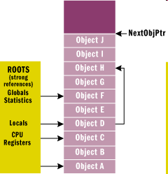
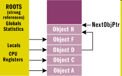
.
It can be seen that memory areas (objects) which were not referred to have disappeared, and the references now point to the new addresses and the pointer that identifies the location of the free area has moved to a lower address (that is, the free contiguous memory has grown).
IV.1.3. Platform independence
Some computers have already left their initial metal box, now we take them with us everywhere in our pockets or we wear them as clothing or accessories. In the case of such computers (which are not called computer anymore: telephone, e-book reader, tablet, media player, glasses, car), manufacturers aim at minimizing consumption besides the relatively smaller computational capacity, since the power of some 100 W necessary for their functioning is not available. The processors made by Intel (and their secondary manufacturers) rather focused on computational capacity and thus mobile devices with batteries are assigned with CPUs made by other manufacturers (ARM, MIPS, etc.). The task of program developers has become more complex: for each CPU (and platform) the application should (have been) developed. It seemed appropriate to create one run-time environment for each platform and then to create applications only once and to compile them to some intermediate code in order to protect intellectual products. This was correctly realized by Sun Microsystems when they created from the languages C and C++ the Java language, which has a simple object model and has no pointers. From Java the application is compiled to bytecode, which is run on a virtual machine (Java VM) or it is translated into native code and is runnable. Nowadays many well-known platforms use the language which has now become the property of Oracle: such an example is the Android operating system supported by Google. Obviously where there is a trademark, there is suing as weel: Oracle did not agree to use the name Java because “its intellectual rights were consciously violated”. The same happened to Microsoft in the case of Java integrated to Windows: current Windows editions do not contain Java support, JRE (the run-time environment) or JDK (the development kit) must be downloaded from the website of Oracle. In the PC world, there is an intermediate stage even without this: the 32 bit operating system cannot handle 4 GB memory. AMD developed the 64 bit instruction set extension, which was later integrated by Intel too. Since XP, Windows can be bought with two types of memory handling: 32 bit for earlier PCs with less than 4 GB memory and 64 bit for PCs with newer CPU and at least 4 GB memory. The 64 bit version runs the earlier, 32 bit applications with the help of emulation (WoW64 – Windows on Windows). When a program is complied with Visual Studio 2005 or a newer (2008, 2010, 2013) version under a 64 bit operating system, we can choose mode x64, then we get a 64 bit application. Thus, there was a need for the ability of running a program on both configurations (x86, x64) and all Windows operating system versions (XP,Vista, 7,8) even if it is not known at the moment of compiling which environment we will have later but we do not want to make more exe files. This requirement can only be fulfilled with the insertion of an intermediate running/compiling level. For bigger programs, it might be necessary that more people be involved in the development, probably with different programming languages. Given the intermediate level, it is also possible: each language compiler (C++, C#, Basic, F# etc.) compiles to this intermediate language, then the application is compiled from this to a runnable one. The intermediate language is called MSIL, which is a stack-oriented language similar to machine code. The first two letters of MSIL refers to the name of the manufacturer and later it was changed to CIL (Common Intermediate Language), which can be seen as the solution of Microsoft for the basic idea of Java.
IV.1.4. Running MSIL code
The CIL code presented in the previous paragraph is transformed into a file with .EXE extension, where it is runable. But this code is not the native code of the processor, so the operating system must recognize that one more step is necessary. This step can be done in two ways, according to the principles used in Java system:
interpreting and running the statements one by one. This method is called JIT (Just In Time) execution. Its use is recommended for the step by step running of the source code and for debug including break points.
generating native code from all statements at the same time and starting it. This method is called AOT (Ahead of Time), and it can be created by the Native Image Generator (NGEN). We use it in the case of well functioning, tested, ready programs (release).
IV.1.5. Integrated development environment
We have not mentioned yet the applied program tools in the development process of the native code that was discussed in the previous paragraph. Initially all the steps were performed by one or more (command line) programs: the developer created/extended/fixed the .C and .H source files with an optional text editor, then the preprocessor, the C compiler and the linker came. When the developer ran the application in debug mode then it meant a new program (the debugger). In case the program contained more source files then only the amended ones had to be recompiled. This was the purpose of the make utility program. When searching among the sources (e.g. searching for in which .H file can a function definition be found) then we could use the grep utility program. Batch files were created for the compiling and those files parametrized the compiler accordingly. In case of a compiling error, the number of the erroneous line was listed on the console then we reloaded the editor, navigated to the erroneous line, we fixed the error and then we restarted the compiler. Once the compiling was completed and the program was started then sometimes it gave erroneous results. In this case we ran it with the debugger then after having the erroneous part found we used the text editor again. This procedure was not effective because of the several needs for restarting the program and the manual information input (line number). On the other hand products with text editor, compiler and runner were developed already in the 70s, 80s, before the PC era. This principal tool was called the integrated development environment (IDE). This IDE type environment was also the Turbo Pascal developed by Borland Inc. that already included a text editor, a compiler and a runner in one program on an 8 bit computer (debugger was not included yet). The program was developed by a certain Anders Hejlsberg who later worked for Microsoft on the development of programming languages. Such languages are J++ and C#. IDE tool for a character screen was created at Microsoft as well: BASIC in DOS was replaced by Quick Basic that already contained an editor and a debugger.
IV.1.6. Controllers, visual programming
Applications that run on operating systems with a graphical user interface (GUI) consist of two parts at least: the code part that contains the algorithm of the program and the interface that implements the user interface (UI). The two parts are logically linked: events (event) happening in the user interface trigger the run of the defined subprograms of the algorithm part (these subprograms are called functions in C type languages). Hence these functions are called “event handler functions” and in the development kit of the operating system (SDK) we can find definitions (in the header files) that are necessary to write them. Initially, programs with a user interface contained also the program parts necessary for the UI: a C language program with 50-100 lines was capable of displaying an empty window in Windows and to manage the “window closing” event (that is, the window could be closed). This time the main part of the development consisted of developing the UI, programming the algorithm could come only after it. In the UI program all coordinates were placed as numbers and after modifying those we could check how the interface looked like. The first similar product of Microsoft (and the recent development tool was named after this) was Visual basic. In the first version of it we could place predefined controls to our form with a GUI (that was basically the user interface of our program that we were developing). A text format code was created from the controls drawn by the user and once needed it could be modified with the embedded text editor then it was compiled before running was initiated. For running the program there was needed a library, consisting the runable parts of the controls. Characteristically because of this small size exe files were created but for the completed program that version of the run-time environment had to be installed in which the program was developed. Visual Basic was later followed by Visual C++ (VC++) and other similar programs, then – based on the example of Office – instead of separate products the development tools were integrated into one product; this was called Visual Studio.
IV.1.7. The .NET framework
The programs that implement the principles discussed till this point were collected by Microsoft into one common software package that could be installed from one file only and they called it .net. During its development several versions of it were published, now at the time when this book is being written version 4.0 is the stable one and 4.5 is the pilot test version. In order to install it we need to know the type of Windows. Different versions have to be installed for each Windows, each CPU and different versions are needed for 32 and 64 bit (see the “Platform independency” chapter).
Parts of the framework:
Common Language Infrastructure (CLI), and its realization the Common Language Runtime (CLR): the common language compiler and run-time environment. MSIL contains a compiler, a debugger and a run-time. It is capable of collecting garbages in the memory (Garbage Collection, GC) and handling exceptions (Exception Handling).
Base Class Library: the library of the basic classes. GUIs can be programmed comfortably in OOP only with well prepared base classes. These cannot be instantiated directly (in most of the cases it is impossible since they are abstract classes). As an example it contains an interface class called “Object” (see later in Section IV.1.10, “Extended data types of C++/CLI”).
WinForms: contols preprepared for the Windows applications, inherited from the Base Class Library. We put these to the form during development and the user interface of our program will be consisted of these. They are language independent contorls and we can use them from any applications according to the syntax of the given language. It is worth mentioning that our program will use not only those controls that were put on the form during development but the program can also create instances from these when running. That is, once putting those controls to the form a piece of the program code is created that runs when the program is initiated. This automatically created source code can be written by us (we can copy it) and it can be run at a later point as well.
Additional parts: these could be the ASP.NET system that supports application development on the web, the ADO.NET that allows access to databases and Task Parallel Library that supports multiprocessor systems. We do not discuss these here because of space restrictions.
IV.1.8. C#
The .NET framework and the pure managed code can be programmed with C# easily. The developer of the language is Anders Hejlsberg. He derived it from the C++ and Pascal languages, kept their advantages, made it simpler and made the usage of more difficult elements (e.g. pointers) optional. It is recommended to amateurs and students in higher education (not for programmers – their universal tools are the languages K&R C and C++). The .NET framework contains a command line C# compiler and we can also download freely the Visual C# Express Edition from Microsoft. Their goal with this is to spread C# (and .NET). Similarly, we can find free books for C# in Hungarian language on the internet.
IV.1.9. Extension of C++ to CLI
The C++ compiler developed by Microsoft can be considered as a standard C++ as long as it is used to compile a native win32 application. However, in order to reach CLI new data types and operations were needed. The statements necessary to handle the managed code (MC) appeared first in the 2002 version of Visual Studio.NET then these were simplified in version 2005. The defined language cannot be considered as C++ because the statements and data types of MC do not fit in C++ standard definition (ISO/IEC 14882:2003). The language was called C++/CLI and it was standardized (ECMA-372). Let us make a note here that usually the goal of standardization is to allow the 3rd party manufacturers to go to the market with the related product, however, in this case it did not happen: C++/CLI can be compiled only by Visual Studio.
IV.1.10. Extended data types of C++/CLI
Variables on the managed heap have to be declared differently than the variables of the native code. The allocation is not automatic because the compiler cannot make a decision instead of us: the native and the managed code can be mixed within one program (only C++/CLI is capable of doing so, the other compilers compile managed code only, e.g. there is no native int type in C#, the Int32 (its abbreviation is int) is already a class). In C++ the class on the managed heap is called reference class (ref class). It can be declared with this keyword the same way as for the native class. E.g. the .NET system contains an embedded “ref class String” type to store and manage accentuated character chains. If we create a "CLR/Windows Forms Application" with Visual Studio, the window of our program will be (Form1) a reference class. A native class cannot be defined within the reference class. The reference class behaves differently compared to the C++ class:
Static samples do not exist, only dynamic ones (that is, its sample has to be created from the program code). The following declaration is wrong: String text;
It is not pointer that points to it but handle (handler) and its sign is ^. Handle has pointer like features, for instance the sign of a reference to a member function is ->. Correct declaration is String ^text; in this case the text does not have any content yet given that its default constructor creates an empty, string with length of 0 (“”).
When creating we do not use the new operator but the gcnew. An example: text=gcnew String(""); creation of a string with length of 0 with a constructor. Here we do not have to use the ^ sign, its usage would be wrong.
Its deletion is not handled by using the delete operator but by giving a value of handle nullptr. After a while the garbage collector will free up the used space automatically. An example: text=nullptr; delete can be used as well, it will call the destructor but the object will stay in the memory.
It can be inherited only publicly and only from one parent (multiple inheritances are possible only with an interface class).
There is the option to create an interior pointer to the reference class that is initiated by the garbage collector. This way, however, we loose the security advantages of the managed code (e.g preventing memory overrun).
The reference class – similarly to the native one – can have data members, methods, constructors (with overloading). We can create properties (property) that contain the data in themselves (trivial property) or contain functions (scalar property) to reach the data after checking (e.g. the age cannot be set as to be a negative number). Property can be virtual as well or multidimensional, in the latest case it will have an index as well. Big advantage of property is that it does not have parenthesis, compared to a native C++ function that is used to reach member data. An example: int length=text->Length; the Length a read only property gives the number of the characters in the string.
Beside the destructor that runs when deleting the class (and for this it can be called deterministic) can contain a finalizer() method which is called by the GC (garbage collector) when cleaning the object from the memory. We do not know when GC calls the finalizer that is why we can call it non-deterministic.
The abstract and the override keywords must be specified in each case when the parent contains virtual method or property.
All data and methods will be private if we do not specify any access modifier.
If the virtual function does not have phrasing, it has to be declared as abstract: virtual type functionname() abstract; or virtual type functionname() =0; (the =0 is the standard C++. the abstract is defined as =0). It is mandatory to override it in the child. If we do not want to override the (not purely) virtual method, then we can create a new one with the new keyword.
It can be set at the reference class that no new class could be created from it with inheritance (with overriding the methods), and it could be only instantiated. In this case the class is defined as sealed. The compiler contains a lot of predefined classes that could not be modified e.g. the already mentioned String class.
We can create an Interface class type for multiple inheritances. Instead of reference we can write an interface class/struct (their meaning is the same at the interface). The access to all the members of the interface (data members, methods, events, properties) is automatically public. Methods and properties cannot be expanded (mandatorily abstract), while data can only be static. Constructors cannot be defined either. The interface cannot be instantiated, only ref/value class/struct can be created from it with inheritance. Another interface can be inherited from an interface. A derived reference class (ref class) can have any interface as base class. The interface class is usually used on the top of the class hierarchy, for example the Object class that is inherited by almost all.
We can use value class to store data. What refers to it is not a handle but it is a static class type (that is, a simple unspecified variable). It can be derived from an interface class (or it can be defined locally without inheritance).
Beside function pointers we can define a delegate also to the methods of a (reference) class that appears as a procedure that can be used independently. This procedure is secured, and errors are not faced that cause a mix up of the types and is possible with pointers of a native code. Delegate is applied by the .NET system to set and call the event handler methods, that belong to the events of the controls.
In the next table we sum up the operations of memory allocation and unallocation:
|
Operation |
K&R C |
C++ |
Managed C++ (VS 2002) |
C++/CLI (VS 2005-) |
|---|---|---|---|---|
|
Memory allocation for the object (dynamic variable) |
|
|
|
|
|
Memory unallocation |
|
|
Automatic, after |
<- similarly as in 2002 |
|
Referring to an object |
Pointer ( |
Pointer ( |
|
Pointer ( Handle ( |
IV.1.11. The predefined reference class: String
The System::String class was created on the basis of C++ string type in order to store text. Its definition is: public sealed ref class String. The text is stored with the series of Unicode characters (wchar_t) (there is no problem with accentuated characters, it is not mandatory to put an L letter in front of the constant, the compiler “imagines” that it is there: L”cat” and “cat” can be used as well). Its default constructor creates a 0 length (“”) text. Its other constructors allow that we create it from char*, native string, wchar_t* or from an array that consists of strings. Since the String is a reference class, we create a handle (^) to it and we can reach its properties and methods with ->. Properties and methods that are often used:
String->Length length. An example: s=”ittykitty”; int i=s->Length; after the value of i will be 9
String[ordinal number] character (0.. as by arrays). An example: value of s[1] will be the ‘t’ character.
String->Substring(from which ordinal number, how many) copying a part. An example: the value of s->Substring(1,3) will be ”tty”.
String->Split(delimiter) : it separates the string with the delimiter to the array of words that are contained in it. An example: s=”12;34”; t=s->Split(‘;’); after t a 2 element array that contains strings (the string array has to be declared). The 0. its element is “12”, and the 1. its elements is “34”.
in what -> IndexOf(what) search. We get a number, the initiating position of the what parameter in the original string (starting with 0 as an array index). If the part was not found, it returns -1. Note that it will not be 0 because 0 is a valid character position. As an example: with the s is “ittykitty”, the value of s->IndexOf(“ki”) will be 4, but the value of s->IndexOf(“dog”) will be -1.
Standard operators are defined: ==, !=, +, +=. By native (char*) strings the comparing operator (==) checks whether the two pointers are equal, and it does not check the equality of their content. When using String type the == operator checks the equality of the contents using operator overloading. Similarly, the addition operator means concatenation. As an example: the value of s+”, hey” will be “ittykitty, hey”.
String->ToString() exists as well because of inheritance. It does not have any pratical importance since it returns the original string. On the other hand, there is no method that converts to a native string (char*). Let us see a function as an example that performs this conversion:
char * Managed2char(String ^s) { int i, size=s->Length; char *result=(char *)malloc(size+1); // place for the converted string memset(result,0,size+1); // we fill the converted with end signs for (i=0; i<size;i++) // we go through the characters result[i]=(char)s[i]; // here we will got a warning: s[i] //stored on 2 bytes unicode wchar_t type character. //Converting ASCII from this the accents will disappear return result; // we will return the pointer to the result }
IV.1.12. The System::Convert static class
We store our data in variables with a type that was chosen for their purpose. For example in case we have to count the number of vehicles passing a certain point of the road per hour, we usually use the int type even if we are aware that its value will never be negative. The negative value (that can be given to the variable because it is signed) can be used in this example to mark an exception (no measuring happened yet, an error occurred etc.). The int (and the other numeric types also) stores the numbers in the memory in binary format, allowing this way performing arithmetic operations (for instance addition, substraction) and calling mathematical functions (e.g. sqrt, sin).
When the user input happens (our program asks for a number), the user will type characters. Number 10 is typed with a ‘1’ and ‘0’ character and from this a string is created: “10”. If we would like to add 20 to this and it was also entered as a string then the result will be “1020” because the “+” operator of the String class copies strings after each other. When using the scanf function of the native Win32 code and the cin standard input stream, if the input was put into numeric type, conversion will happen when reading to the type that is specified in the scanf format argument or after the cin >> operator. In case of the predefined input controls of windows it does not work like this: their output is always String type. Similarly, we always have to create String type for the output because on our controls we can display only this type. Also text files that are used to establish communication between programs (export/import) consist of strings in which numbers or other data types (date, logical, currency) can be as well. The System namespace contains a class called Convert. The Convert class has numerous overloaded static methods, which help the data conversion tasks. For performing the most common text <-> number conversions the Convert::ToString(NumericType) and the Convert::ToNumericType(String) methods are defined. For example, if in the above example s1=”10” and s2=”20”, then we add them considered as integers in the following way:
int total=Convert::ToInt32(s1)+Convert::ToInt32(s2);
In case s1 or s2 cannot be converted to a number (for example one of them is of 0 length or it contains an illegal character) an exception arises. The exception can be handled with a try/catch block. In case of real numbers we have to pay attention to one more thing: these are the region and language settings. As known, in Hungary the decimal part of numbers are separated from the integer with a comma: 1,5. On the other hand, in English speaking countries point is used for this purpose:1.5. In the source code of the C++/CLI program we always use points in case of real numbers. The Convert class, however, performs the real <-> string conversion according to the region and language settings (CultureInfo). The CultureInfo can be set for the current program, if for example we got a text file that contains real numbers in English format. The next program part sets its own culture information so that it could handle such a file:
// c is the instance of the CultureInfor reference class
System::Globalization::CultureInfo^ c;
// Like we were in the USA
c = gcnew System::Globalization::CultureInfo("en-US");
System::Threading::Thread::CurrentThread->CurrentCulture = c;
// from now onwards in the program the decimal separator is the point, the list delimiter is the comma
The methods of the Convert class can appear also in the methods of the data class. For example the instance created by the Int32 class has a ToString() method to convert to a string and a Parse() method to convert from a string. These methods can be parameterized in several ways. We often use hexadecimal numbers in computer/hardware related programs. The next example communicates with an external hardware with the use of strings containing hexadecimal numbers through a serial port:
if (checkBox7->Checked) c|=0x40;
if (checkBox8->Checked) c|=0x80;
sc="C"+String::Format("{0:X2}",c);// A 2 character hex number is created from the byte type c. C is the command;
//if the value of c was 8: “C08” will be the output, if c was 255 "CFF”.
serialPort1->Write(sc); // we sent it to the hardware
s=serialPort1->ReadLine(); // the answer was returned
// let us convert the answer to an integer
status = Int32::Parse(s, System::Globalization::NumberStyles::AllowHexSpecifier);
IV.1.13. The reference class of the array implemented with the CLI array template
In programming the array is an often used data structure with basic algorithms. Developers of .NET developed a generic array definition class template. With help of this – like a producer tool - the user can define a reference class from the required basic data type using the (<>) sign introduced in C++ to mark templates. It can be used for multidimensional arrays as well. Accessing the elements in the array can happen with the integer number (index) put into the traditional square brackets, that is with the [ ] operator.
Declaration: cli::array<type, dimension=1>^ arrayname, the dimension is optional; in this case its value is 1. The ^ is the sign of the ref class, the cli:: is also omissible, if we use at the beginning of our file the using namespace cli; statement.
We have to allocate space for the array with the gcnew operator before using – since it is a reference class when declaring a variable only the handle is created, and it is not pointing to anywhere. We can make the allocation in the declaration statement as well: we can list the elements of the array between { } as used in C++.
Array’s property: Length gives the number of elements of the onedimensional array. For arrays passed to a function we do not have to pass the size, like in the basic C. The size can be used in the loop statement, which does not address out from the array:
for (i=0; i<arrayname->Length; i++)….
For the basic array algorithms static methods were created, and those are stored in the System::Array class:
Clear(array, from where, how many) deletion. The value of the array elements will be 0, false, null, nullptr (depending on the base type of the array),
Resize(array, new size) in case of resizing (expanding) after the old elements it fills the array with the values used with Clear().
Sort(array) sorting the elements of the array. It can be used by default to order numerical data in ascendant order. We can set keys and a comparing function to sort any type data.
CopyTo(target array, starting index) copying elements. Note: the = operator duplicates the reference only. If an element of the array is changed, this changed element is reached using the other reference as well. Similarly, the == oparetor that the two references are the same but it does not compare the elements themselves.
If the type from which we create the array is another reference class (e.g. String^) then we have to set it in the definition. After creating the array we have to create each element one after the other because by default it would contain nullptrs. An example: String^ like an array element with initial value setting. If we do not list the 0 length strings, the array elements would have been nullptrs
array<String^>^ sn= gcnew array<String^>(4){"","","",""};
In the next example we create lottery numbers in an array then we check them whether they can be used in the game: not to have two identical ones. In order to do this we sort them so that we had to check only the neighbouring elements and we could list the result in ascendent order:
array<int>^ numbers; // managed array type, reference
Random ^r = gcnew Random();// random number generator instance
int piece=5, max=90,i; // we set how many numbers we need and the highest number.
//It could be set as an input after conversion.
numbers = gcnew array<int>(piece); // managed array on the heap created
for(i=0;i<numbers->Length;i++)
numbers[i]=r->Next(max)+1;// the raw random numbers are in the array
Array::Sort(numbers); // with the embedded method we set the numbers in order
// check: two identical next to each other?
bool rightnumber=true;
for (i=0;i<numbers->Length-2;i++)
if (numbers[i]==numbers[i+1]) rightnumber=false;
IV.1.14. C++/CLI: Practical realization in e.g. in the Visual Studio 2008
If we would like to create a program with CLR (that is, in .NET with windows) in Visual Studio we have to choose one of the “Application” elements of the CLR category in the new element wizard. The CLR console looks like the ”Win32 console app”, that is, it has a command line interface. Therefore we should not choose the console but the ”Windows Forms Application”. In this case the window of our program that is the container object called Form1 will be created and its code will be in the Form1.h header file. The Form Designer will place the code of the drawn controls here (and it puts a comment ahead of it saying that we should not modify the code, of course in certain cases the amendment is necessary). In the attached figure you can see the element to be selected:
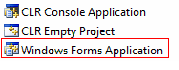
After making our selection, the folder structure of our project is created with the necessary files in it. Now we can already place controls on the form. In the “Solution Explorer” window we can find for the source files and we can modify all of them. In the next figure you can see a project that has just been started:
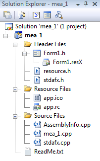
Our program is in Form1.h (it has a form icon). Usually there is code placed into stdafx.h too. In the main program (mea_1.cpp) we should not modify anything. Using the “View/Designer” menuitem, we can select the graphical editor, while with the “View/Code” menuitem the source program. After selecting the “View/Designer” menuitem our window will look like this:
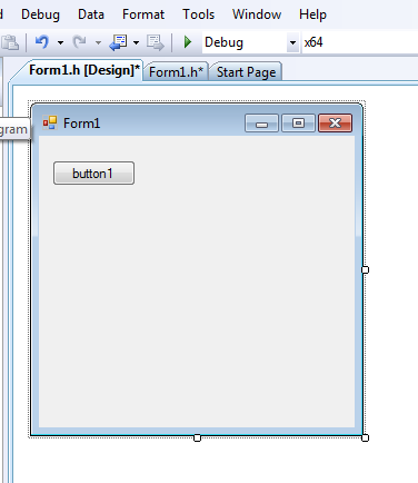
After selecting the “View/Code” menuitem our window will look like this:
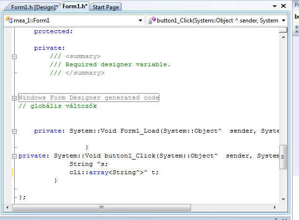
Selecting the “View/Designer” menuitem we will need the Toolbox where the additional controls can be found (the toolbox contains additional elements only in designer state). In case it is not visible we can set it back with the “View/Toolbox” menuitem. The toolbox contains a case-sensitive help as well: leaving the cursor on top of the controls we will get a short summary of the use of the control. See the next figure where we selected the label control:
Selection of the control happens with the usual left mouse button. After this the bounding rectangle of the control will be drawn on the form if we chose a visible control. The non-visible controls (e.g. timer) can be placed in a separated band at the bottom of the form. When the drawing is done an instance of the control is put to on the form with an automatically given name. In the figure we selected the “Label” control (upper case: type), if we draw the first of this control, the developing environment will name it “label1” (lower case: instance). After drawing the controls if needed, we can set their properties and the functions that are related to their events. After selecting the control and with right mouse click we can achieve the setting in the window, opened with the “Properties” menuitem. It is important to note that these settings refer to the currently selected control and the properties windows of the certain controls differ from each other. On the next figure we select the “Properties” window of the label1 control:
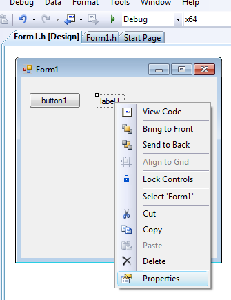
After this we can set the properties in a separate window:
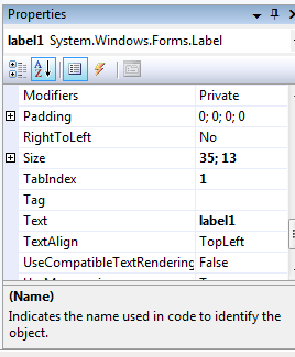
The same window serves for selecting the event handlers. We have to click on the blitz icon ( ) to define the event handlers. In this case all the reacting options will appear that are possible for all the events of the given control. In case the right side of the list is empty then the control will not react to that event.
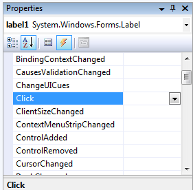
In the example the label1 control does not react when clicking on it (the label control can handle the click event but it is not common to use the control this way). A function can be added to the list in two ways: if we would like to run an already existing function when the event of the control happens (and its parameters equal to the event parameters), then we can choose the function name from the drop down list. If it does not exist then clicking on the empty area the header of a new function is created and we will reach the code editor. Each control has a default event (for example click is the default event of the button), clicking twice on the control in the designer window we will reach the code editor of the event. If such a function does not exist yet its header and an association are created. We have to be aware that the control does not work without its association! It is a typical problem to write the button1_Click function, setting the parameters correctly but without associating them. In this case – after compiling without errors – the button does not react when clicking on it. The button1 will react only if the “Click” row in the events window contains the button1_Click name.
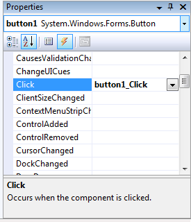
IV.1.15. The Intellisense embedded help
As we saw it in the previous figures, a control can have a lot of properties. We can use the property names in the text of the program, but since they are considered as identifiers they have to equal from character to character to the property name as set in the definition, considering case sensitivity as well. The names of the properties are often very long (for example UseCompatibleTextRendering). The programmer has to type these without mistake. The text editor contains some help: after the name of the object (button1) typing the operator that refers to the data member (->) it creates a list from the possible properties. It displays them in a short menu, we can select the ones we need with the cursor control arrows or with the mouse, then it adds the chosen name to the text of our program pushing the tab key. The help list will appear also if we start to type the name of the property. Visual Studio stores these control properties in a big size .NCB extension file and if we delete it (e.g we transfer a source file to another computer via pen drive), once opening it, it will be regenerated. Intellisense does not work in certain cases: if our program has syntax errors, and the number of opening curly brackets does not equal to the closing curly brackets, then it will stop. Similar to this it does not work in Visual Studio 2010, if we write a CLR code. In the next figure we would like to change the label7->Text property, because of the high number of properties we type the T letter then we select Text with the mouse.
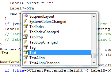
IV.1.16. Setting the type of a CLR program.
As we already mentioned previously, C++/CLR is capable of developing mixed mode programs (native+managed). In case we use settings described in the previous section, our program will have purely managed code, the native code cannot be compiled. At the beginning it is worth to start with these settings because this way the window and the controls of our program will be usable. We can make these settings in the project properties (we select the project then right click and “Properties”). Be aware that it does not refer to the top level solution but to the properties of the project that is below the solution.
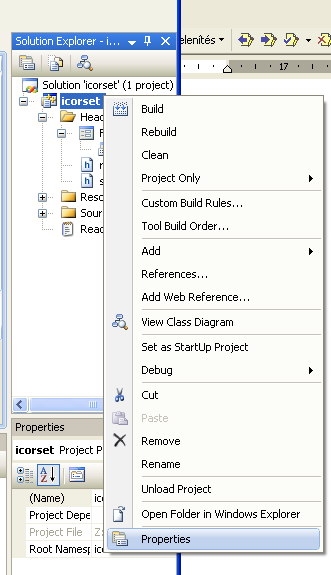
In the "Property Pages" window in the line “Common Language Runtime Support" we can set whether it should be native/mixed/purely managed code. We can choose from 5 setting types:
The meanings of the settings are as follows:
"No common Language Runtime Support" – there is no managed code. It is the same if we create a Win32 console application or a native Win32 project. With this setting it is not capable of compiling the parts of the .NET system (handles, garbage collector, reference classes, assemblies).
"Common Language Runtime Support" – there is native and managed code compiling as well. With this setting we can create mixed mode programs, that is, if we started to develop our program with the default window settings and we would like to use native code data and functions, then we have to set the drop down menu to this item.
"Pure MSIL Common Language Runtime Support" – purely managed code compiling. The default setting of programs created from the “Windows Form Application”. This is the only possible setting of C# compiler. Note: this code type can contain native code data that we can reach through managed code programs.
"Safe MSIL Common Language Runtime Support" – it is similar to the previous one but it cannot contain native code data either and it allows the security check of the CRL code with a tool created for this purpose (
peverify.exe)."Common Language Runtime Support, Old Syntax" – this also creates a mixed code program but with Visual Studio 2002 syntax. (_gc new instead of gcnew). This setting was kept to ensure compatibility with older versions, however, it is not recommended to be used.
IV.2. The window model and the basic controls
IV.2.1. The Form basic controller
Form could not be added from the toolbox, it is created with a new project. By default it creates an empty, rectangle shape window. Its settings can be found in the properties, e.g. Text is its header and by default the name of the control (if this is the first form then it will be Form1) will be added into it. We can reach it from here or from the program as well ((this->Text=…) because in the Form1.h can be used the instance of the reference class of our form (inherited from the Form class), and we can refer to this instance with this pointer within our program. From the property settings (as well) a program part is created at the beginning of form1.h in a separate section:
#pragma region Windows Form Designer generated code
/// <summary>
/// Required method for Designer support - do not modify
/// the contents of this method with the code editor.
/// </summary>
// button1
this->button1->Location = System::Drawing::Point(16, 214);
this->button1->Name = L"button1";
this->button1->Size = System::Drawing::Size(75, 23);
this->button1->TabIndex = 0;
this->button1->Text = L"button1";
this->button1->UseVisualStyleBackColor = true;
this->button1->Click += gcnew System::EventHandler(this, &Form1::button1_Click);
IV.2.2. Often used properties of the Form control
Text – title of the form. This property can be found at each control that contains text (as well).
Size – the size of the form, by default in pixels. It contains the Width and Height properties that are directly accessible. Also the visible controls have these properties.
BackColor – color of the background. By default it has the same color as the background of the controls defined in the system (System::Drawing::SystemColors::Control). This property will be important if we would like to delete the graphics on the form because deletion means filling with a color.
ControlBox – the system menu of the window (minimalizer, maximalizer buttons and windows menu on the left side). It can be enabled (by default) and disabled.
FormBorderStyle – We can set here whether our window can be resized or it should have a fix size or whether it had a frame or not.
Locked – we can prohibit resizing and movement of the window with the help of this.
AutoSize – the window is able to change its size aligning to its content
StartPosition – when starting the program where should the form appear on the Windows desktop. Its application: if we use a multiscreen environment, then we can set the x,y coordinates of the second screen, our program will be lunched there then. It is useful to set this property in a conditional statement because in case the program is lunched in one screen only the form will not be visible.
WindowState – we can set here whether our program would be a window (Normal), whether it would run full screen (Maximized) or whether it would run in the background (Minimized). Of course, like any of the other properties, it is reachable during run-time as well, that is, if the program lunched in the small window would like to maximalize itself (for example because it would like to show many things) then we have an option for this setting as well: this->WindowState=FormWindowState::Maximized;
IV.2.3. Events of the Form control
Load – a program part that appears when starting the program before displaying it. Load is the default event of the Form control, that is, when double clicking on its header in the Designer its handler function is placed in the editor. This function as usual can fill in the role of an initializer since it runs once when launching the program. We can set values to the variables, we can create the necessary dynamic variables, and we can change title on our other controls (if we have not already done ), we can also set the size of the form dynamically etc.
As an example let us see the Load event handler of the program of the quadratic equation:
private: System::Void Form1_Load(System::Object^ sender, System::EventArgs^ e) {
this->Text = "quadratic";
textBox1->Text = "1"; textBox2->Text = "-2"; textBox3->Text = "1";
label1->Text = "x^2+"; label2->Text = "x+"; label3->Text = "=0";
label4->Text = "x1="; label5->Text = "x2="; label6->Text = "";
label7->Text = ""; label8->Text = "";
button1->Text = "Solve it";
if (this->ClientRectangle.Width < label3->Left + label3->Width) // the form is not wide enough
this->Width = label3->Left + label3->Width + 24;
if (this->ClientRectangle.Height < label8->Top + label8->Height)
this->Height = label8->Top + label8->Height + 48; // it is not high enough
button1->Left = this->ClientRectangle.Width - button1->Width-10; // pixel
button1->Top = this->ClientRectangle.Height - button1->Height - 10;
}
In the above example after setting the initial values we set the titles then we set the size of the form to a value that the whole equation and the results (label3 was the right-most control and label8 was at the bottom of the form) were visible.
In case we find in this function that running of the program does not make sense (we would process a file but we could not find it, we would like to communicate with a hardware but we could not find it, we would like to use the Internet but we do not have connection etc.) then after displaying a window of an error message we can leave the program. Here comes a hardware example:
if (!controller_exist) {
MessageBox::Show("No iCorset controller.",
"Error",MessageBoxButtons::OK);
Application::Exit();
} else {
// controller exist, initialize the controller.
}
Let us pay attention to a thing: the Application::Exit() does not leave the program immediately, it puts a message to the Windows message queue for us to warn about leaving the program. That is, the program part after if… will run also, moreover the window of our program will show up for a second before closing it. If we would like to avoid the run of the further program part (we would communicate with the hardware that does not exist), then let us do it in the else branch of the if statement and the else branch should reach the end of the Load function. This way we can guarantee that the program part that supposedly caused the error will not run.
Resize – An event handler that runs when resizing our form (minimalizing, maximalizing, setting it to its normal size could be also considered here). It runs when loading the program, this way the increase of the form size from the previous example could have been mentioned here as well, and in this case the form could not be resized to smaller in order to ensure the visibility of our controls. In case we have a graphic which size depens on the window size, then we can resize it here.
Paint – the form has to be repainted. See the examples in the “The usage of GDI+” chapter (Section IV.4.1, “The usage of GDI+”).
MouseClick, MouseDoubleClick – we click once or we double click on the Form with the mouse. In case we have other controls on the form then this event runs if we do not click on neither of the controls just on the empty area. In one of the arguments of the event handler we got the handle to the reference class
System::Windows::Forms::MouseEventArgs^ e
The referenced object contains the coordinates (X,Y) of the click beside others.
MouseDown, MouseUp – we clicked or released one of the mouse buttons on the Form.The Button propety of the MouseEventArgs contains which button was clicked or released. The next program part saves the coordinates of the clicks into a file, this way for example we can create a very basic drawing program:
// if save is set and we pushed the left button
if (toolStripMenuItem2->Checked && (e->Button == System::Windows::Forms::MouseButtons::Left)) {
// we write the two coordinates into the file, x and y as int32
bw->Write(e->X); // we write int32
bw->Write(e->Y); // that is 2*4 byte/point
}
MouseMove: - the function running when moving the mouse. It works independently from the buttons of the mouse. In case our mouse is moved over the form, its coordinates can be read. The next program part displays these coordinates in the title of the window (that is, in the Text property), of course after the needed conversions:
private: System::Void Form1_MouseMove(System::Object^ sender, System::Windows::Forms::MouseEventArgs^ e) {
// coordinates into the header, nobody looks at those ever
this->Text = "x:" + Convert::ToString(e->X) + " y=" + Convert::ToString(e->Y);
}
FormClosing – our program got a Terminate() Windows message for some reason. The source of the message could be anything: the program itself with Application::Exit(), the user with clicking on the “close window”, or the user with the Alt+F4 key combination, we are before stopping the operating system etc. When this function runs the Form is closed, its window disappears, resources used by it will be unallocated. In case our program decides that this is not possible yet, the program stop can be avoided by setting the Cancel member of the event’s parameter to true, and the program will run further. The operating system however, if we would like to prevent it from stopping, it will close our program after a while. In the next example the program let itself to be closed only after a question appearing in a dialog window:
void Form1_FormClosing(System::Object^ sender, System::Windows::Forms::FormClosingEventArgs^ e) {
System::Windows::Forms::DialogResult d;
d=MessageBox::Show("Are you sure that you would like to use the airbag?”,
" Important security warning ", MessageBoxButtons::YesNo);
if (d == System::Windows::Forms::DialogResult::No) e->Cancel=true;
}
FormClosed – our program is already in the last step of closure process, the window do not exist anymore. There is no way back from here, this is the last event.
IV.2.4. Updating the status of controls
After the running of the event handlers (Load, Click) the system updates the status of controls so that they are already in the new, updated state for the next event. However, let’s have a look at the following sample program part that writes increasing numbers into the form’s title bar. It can be placed for example into the button_click event handler:
int i;
for (i=0;i<100;i++)
{
this->Text=Convert::ToString(i);
}
During the running of the program (apart from the speed problem) there is no change in the form’s title. Though Text property was rewritten, the control still shows the old content. It will be changed only once, when the given event handler function terminates. But then „99” will appear in the control. In case of longer operations (image processing, large text files) it would be good to somehow inform the user about how the program proceeds, showing the current status, otherwise one might suppose that the program has stopped responding. Function call Application::DoEvents() serves exactly this purpose. It updates the current status of the controls: in our example this function will replace the form’s title. Unfortunately, from this we cannot see anything, we can read the numbers only if we build an awaiting time (Sleep) as well into the loop:
int i;
for (i=0;i<100;i++)
{
this->Text=Convert::ToString(i);
Application::DoEvents();
Threading::Thread::Sleep(500);
}
The parameter of the Sleep() function is the waiting time in milliseconds. The slow process was simulated by this. In case we need algorithm components recurring periodically, Timer control should be used (see Section IV.2.22, “Control used for timing: Timer”).
IV.2.5. Basic controls: Label control

The simplest control is the Label which displays text. It’s String ^ type property called Text includes the text to be displayed. By default its width aligns to the text to be displayed (AutoSize=true). In case we display text with the help of it, its events (eg. Click) are normally not used. By default the Label has no border (BorderStyle=None), but it can be framed (FixedSingle). The background color can be found in BackColor property, the text color in ForeColor property. In case we would like to remove the displayed text, we have two choices: we either set the logical type property called Visible to false, in this case the Text property does not change, but the control is not visible, or we set the Text property to an empty string with length 0 (””).
All visible controls have this property called Visible. By setting the property to false, the control disappears, by setting it to true, the control will be visible again. In case we are sure that the control’s label will be different at the next display, it is practical to use the ‘empty string’ version, since in this case the new value appears immediately after the assignment; while in case of the other version ‘Visible property’ a new allowing program line is needed as well.
IV.2.6. Basic controls: TextBox control

TextBox control can be used for entering text (String^) (in case we need to enter numbers, we use the same control, but in this case the processing starts with a conversion). The Text property contains the text, which can be rewritten from the program and the user can also change it while the program is running. The already mentioned Visible property appears here as well as the Enabled property is available too. By setting Enabled to false, the control is visible on the form, however appears in gray and cannot be used by the user: one can neither change nor click on it. For example, the command button “Next” in an installation process has the same state until the license agreement is not accepted.
TextBox has a default event as well: it is TextChanged, which runs after each and every change (per character). In case of multi-digit numbers, data with more than one characters or in case of more input data (in several TextBoxes) we usually do not use it, since it would be pointless. For example, the user has to enter his name into the TextBox and the program stores it in a file. It would be unnecessary to write all the current content into a file in case each of the characters, since we do not know what the last character will be. Instead, we wait until editing is over, data entry is ready (maybe there are more TextBoxes in our form), and the user can give a signal by pressing a properly named (ready, save, processing) command button meaning that text boxes include the program’s input data.
Unlike the other controls that have Text property, where the Designer writes the control’s name into the Text property, it does not happen here, Text property remains empty. It can be set to multiline by switching the MultiLine property to true. Then line feeds appear in the Text, and the lines can be found in the Lines property just like the elements of a string array. Some programmers use TextBox control for output as well by setting ReadOnly property to true. In case we do not want to write back the entered characters, we can switch the TextBox to password input mode by setting UseSystemPasswordChar property to true. We have already seen the function running when starting the quadratic equation program; now let’s have a look at the calculation part. The user has written in the TextBoxes the coefficients (a,b,c) and clicked on the “solve” button. Our first job is to get data from the TextBoxes by using conversion. Then the next step is the calculation and the displaying of results.
double a, b, c, d, x1, x2, e1, e2; // local variables
// in case we forget to give values to any of the variables -> error
a = Convert::ToDouble(textBox1->Text); // String -> double
b = Convert::ToDouble(textBox2->Text);
c = Convert::ToDouble(textBox3->Text);
d = Math::Pow(b,2) - 4 * a * c; // the method for exponentiation exists as well
if (d >= 0) // real roots
{
x1=(-b+Math::Sqrt(d))/(2*a);
x2=(-b-Math::Sqrt(d))/(2*a);
label4->Text = "x1=" + Convert::ToString(x1);
label5->Text = "x2=" + Convert::ToString(x2);
// checking
e1 = a * x1 * x1 + b * x1 + c; // this way we typed less than in Pow
e2 = a * x2 * x2 + b * x2 + c;
label6->Text = "...=" + Convert::ToString(e1);
label7->Text = "...=" + Convert::ToString(e2);
}
IV.2.7. Basic controls: Button control

Button control denotes a command button that “sags” when clicking on it. We use command button(s) if the number of currently selectable functions are low. The function can be complicated as well, in this case a long function belongs to it. Button control supports the usual properties of visible controls: its caption is Text, its event is Click, which runs when clicking on the button. This is its default and commonly used event. From the event handler’s parameters the coordinates of the click cannot be told. The header of the event handler is:
private: System::Void button1_Click(System::Object^ sender, System::EventArgs^ e) {
}
Button control gives an opportunity to apply the nowadays so fashionable shortcut icon operation by using small graphics instead of captions. To do this, the following steps are needed: we load the small graphic to a Bitmap type variable, we set the Button’s sizes to the sizes of Bitmap, finally, we store the reference of the Bitmap type variable in the Image property of the button as it happened in the example below: the image called “service.png” appears in the command button called “button2”.
Bitmap^ bm;
bm=gcnew Bitmap("service.png");
button2->Width=bm->Width;
button2->Height=bm->Height;
button2->Image=bm;
IV.2.8. Controls used for logical values: CheckBox

Text property of the CheckBox control is the text (String^ type), written next to it. Its bool type property is the Checked, which is true in case it is checked. CheckedState property can take up three values: apart from ‘on’ and ‘off’ it has a third, middle value as well, which can be set up only from the program, when it is running, however it is considered to be checked. In case there are more CheckBoxes in a Form, these are independent of each other: we can set any of them checked or unchecked. Its event: CheckedChanged occurs when the value of the Checked property changes.
The sample program below is a part of an interval bisection program: when switching on the checkbox called “Stepwise”, one step will be completed from the algorithm, when switching it off, the result is provided within one loop. If we started to make the program running stepwise, the checkbox cannot be unchecked: further counting has to be performed stepwise.
switch (checkBox1->Checked)
{
case true:
checkBox1->Enabled = false;
step();
break;
case false:
while (Math::Abs(f(xko)) > eps) step();
break;
}
write();
IV.2.9. Controls used for logical values: RadioButton

RadioButton is a circular option button. It is similar to the CheckBox, but within one container object (such as Form: we put other objects in it) only one of them can be checked at the same time. It was named after the old radio containing waveband switch: when one of the buttons was pressed, all the others were deactivated. When one of the buttons is marked/activated by the circle (either by the program: Checked = true, or by the user clicking on it), the previous button (and all the others) becomes deactivated (its Checked property changes to false). We store the text, which is next to the circle in the control’s Text property. A question might be raised: if only one RadioButton can be active at the same time, then what if we have to choose from two option lists at the same time using RadioButtons? The answer is simple: we can have one active RadioButton per one container object, therefore, we have to place some container objects on the form.
IV.2.10. Container object control: GroupBox

GroupBox is a rectangular frame with text (Text, String^ type) on its top left line. We placed controls in it, which are framed. On the one hand, it is aesthetic, as the logically related controls appear within one frame, on the other hand it is useful for RadioButton type controls. Furthermore, controls appearing here can be moved and removed with a single command by customizing the appropriate property of GroupBox. The example below shows marking: we can see the entry and processing of a small number of discrete elements:
groupBox1->Text="ProgDes-I"; radioButton1->Text="excellent"; radioButton2->Text="good"; radioButton3->Text="average";// no other marks can be received here … int mark; if (radioButton1->Checked) mark = 5; if (radioButton2->Checked) mark = 4;
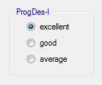
IV.2.11. Controls inputting discrete values: HscrollBar and VscrollBar


The two controls that are called scrollbars differ only in direction. They do not have labels. In case we would like to indicate their end positions or their current status, we can do this by using separate label controls. The current value, where the scrollbar is standing, is the integer numerical value found in Value property. This value is located between the values of Minimum and Maximum properties. The scrollbar can be set to the Minimum property, this is its left/upper end position. However, for its right/lower end position we have a formula, which includes the quick-change unit of the scrollbar, called LargeChange property (the value changes this much, when we click on the empty space with the mouse): Value_max=1+Maximum-LargeChange. LargeChange and SmallChange are property values set by us. When moving the scrollbar a Change event is running with the updated value. In the example below we would like to generate 1 byte values (0..255) with the help of three equally sized horizontal scrollbars. The program part for setting the scrollbar properties in the Form_Load event are the following:
int mx; mx=254 + hScrollBar1->LargeChange; // We would like to have 255 in the right position hScrollBar1->Maximum = mx; // max. 1 byte hScrollBar2->Maximum = mx; hScrollBar3->Maximum = mx;
When the scrollbars are changing, we read their value, convert them to a color and write the values to the labels next to the scrollbars as a check:
System::Drawing::Color c; // color variable r = hScrollBar1->Value ; // from 0 to 255 g = hScrollBar2->Value; b = hScrollBar3->Value; c = Color::FromArgb(Convert::ToByte(r),Convert::ToByte(g),Convert::ToByte(b)); label1->Text = "R=" + Convert::ToString(r); //we can also have them written label2->Text = "G=" + Convert::ToString(g); label3->Text = "B=" + Convert::ToString(b);
IV.2.12. Control inputting integer numbers: NumericUpDown
With the help of NumericUpDown control we can enter an integer number. It will appear in Value property, between the Minimum and Maximum values. The user can increase and decrease the Value by 1, when clicking on the up and down arrows. All the integer numbers between the Minimum and Maximum values appear among the values to choose from. Event: ValueChanged is running after every change.
IV.2.13. Controls with the ability to choose from several objects: ListBox and ComboBox


ListBox control offers an arbitrary list to be uploaded, from which the user can choose. Beyond the list, ComboBox contains a TextBox as well, which can get the selected item as well and the user is also free to type a string. This is the Text property of ComboBox. The control’s list property is called Items, which can be upgraded by using Add() method and can be read indexed. SelectedIndex points the current item. Whenever selection changes, SelectedIndexChanged event is running. ComboBox control is used by several controls implementing more complex functions: for example OpenFileDialog. In the example below we fill up the list of ComboBox with elements. When the selection is changed, we put the new selected item in label4.
comboBox1->Items->Add("Excellent");
comboBox1->Items->Add("Good");
comboBox1->Items->Add("Average");
comboBox1->Items->Add("Pass");
comboBox1->Items->Add("Fail");
private: System::Void comboBox1_SelectedIndexChanged(System::Object^ sender, System::EventArgs^ e) {
if (comboBox1->SelectedIndex>=0)
label4->Text=comboBox1->Items[comboBox1->SelectedIndex]->ToString();
}
IV.2.14. Control showing the status of progressing: ProgressBar

With the help of ProgressBar we can give information about the status of the process, how much is still left, the program has not frozen, it is working. We have to know in advance when the process will be ready, when it should reach the maximum. The control’s properties are similar to HScrollBar, however the values cannot be modified with the help of the mouse. Certain Windows versions animate the control even if it shows a constant value. Practically, this control used to be placed in the StatusStrip in the bottom left corner of our window. When clicking on it, its Click event is running, however, it is something we normally do not deal with.
IV.2.15. Control with the ability to visualize PixelGrapic images: PictureBox

This control has the ability to visualize an image. Its Image property contains the reference of the Bitmap to be visualized. Height and Width properties show its size, while Left and Top properties give its distance from the left side and top of the window measured in pixels. It is practical to have the size of the PictureBox exactly the same as the size of the Bitmap to be visualized (which can be loaded from almost all kinds of image files) in order to avoid resizing.
The SizeMode property contains the info about what to do if you need to resize the image: in case of Normal value, there is no resizing, the image is placed to the left top corner. If Bitmap is larger, the extra part will not be displayed. In case of StretchImage value, Bitmap is resized to be as large as the PictureBox. In case of AutoSize option, the size of the PictureBox is resized according to the size of the Bitmap. In the program below we display a temperature map (found in idokep.hu) in the PictureBox control. SizeMode property is preset in the Designer, the size parameters of the images are shown in the label:
Bitmap ^ bm=gcnew Bitmap("mo.png");
label1->Text="PictureBox:"+Convert::ToString(pictureBox1->Width)+"x"+
Convert::ToString(pictureBox1->Height)+" Bitmap:"+
Convert::ToString(bm->Width)+"x"+Convert::ToString(bm->Height);
pictureBox1->Image=bm;
The result of the program above in case SizeMode=Normal is the following:
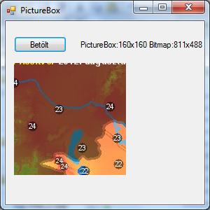
With SizeMode=StretchImage setting the scales do not match either: the map is rectangular, the PictureBox is a square:
In case of SizeMode=AutoSize the PictureBox has increased, but the Form has not. The Form had to be resized manually to reach the following size:
With SizeMode=CenterImage setting: there is no resize, the centre of Bitmap was set into the PictureBox
With SizeMode=Zoom Bitmap is resized by keeping its scales so that it fits into the PictureBox:
IV.2.16. Menu bar at the top of our window: MenuStrip control

In case our program implements so many functions that we would require a large number of command buttons in order to start them, it is practical to group functions hierarchically and settle them into a menu. Imagine for example that if all the functions of Visual Studio could be operated with command buttons, editor window could not fit because of the large number of buttons. The menu starts from the main menu, this is always visible at the top of the program’s window and every menu item can have submenus. The traditional menu includes labels (Text), but newer menu items can show bitmaps as well, or there can be TextBoxes and ComboBoxes used for editing too. We can put a separator among menu items (being not in the main menu) and we can also put a checkbox in front of the menu items. Menu items similarly to command buttons get a unique identifier. The identifier can be typed by us, or similarly to the other controls, it can be named automatically. MenuStrip control appears under the form, but in the meanwhile we can write the name of the menu item in the top corner of our program, or we can choose the automatic name by using the “MenuItem” label. In the figure below we can see the start of menu editing, when we included MenuStrip:
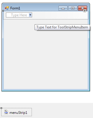
Let’s select a menu item in the menu above:
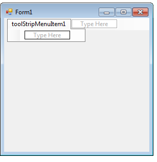
The name of the menu item in the main menu is now toolStripMenuItem1. To the place of the menu item being next to it (in the main menu) let’s type: Help.
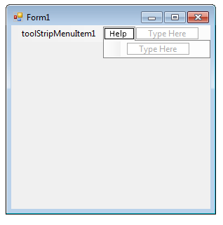
The name of the new menu item is now helpToolStripMenuItem, however its Text property does not have to be set: it is already done. Let’s create three submenu items under MenuItem1 using a separator before the third one:
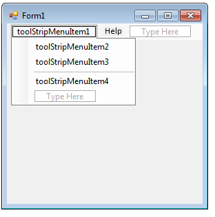
From now programming is the same as in case of buttons: in form_load function we set their labels (Text), then we write the Click event handler methods by clicking on the menuitems in the editor:
private: System::Void toolStripMenuItem2_Click(System::Object^ sender, System::EventArgs^ e) {
// We have to write here what should happen after we have selected the menu item.
}
IV.2.17. The ContextMenuStrip control which is invisible in basic mode

The main menu of the MenuStrip control is always visible. The ContextMenuStrip can only be seen while designing, during running it is only visible if it is visualized from the program. It is recommended to use it with the local menu appearing at the mouse cursor after clicking the right mouse button. We create the items of the menu in Designer, we write the Click event hanler of the menu items in the editor then in the MouseDown or MouseClick event handler of the Form (they have a coordinate parameter) we visualize the ContextMenu.
The program part below contains a ContextMenu with three menuitems:
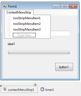
The event control Form_MouseClick looks like this:
private: System::Void Form1_MouseClick(System::Object^ sender, System::Windows::Forms::MouseEventArgs^ e) {
if (e->Button == Windows::Forms::MouseButtons::Right) // only for the right button
contextMenuStrip1->Show(this->ActiveForm, e->X, e->Y); // we show the menu to the Form
}
IV.2.18. The menu bar of the toolkit: the control ToolStrip

The toolkit contains graphical command buttons next to each other. The Image property of the buttons contains the visualized image. Since they are command buttons, they run the Click event when clicking on them. The figure below shows the elements of the toolstrip, with the button contatining the image at the top, which will bear a name starting with toolStripButton:
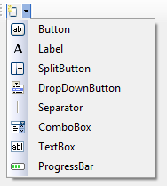
IV.2.19. The status bar appearing at the bottom of the window, the StatusStrip control

A status bar visualises status information, therefore it is useful to create a label and a progressbar for it. The name of the label placed over it starts with toolStripLabel, that of the progressbar will start with toolStripProgressBar. It is not clicked in general, so Click event handlers are not written for it.
IV.2.20. Dialog windows helping file usage: OpenFileDialog, SaveFileDialog and FolderBrowserDialog


Almost all computer programs in which modifications carried out can be saved contain the Open file and Save file functions. Selecting a file to be saved or to be opened is done with the same window type in each software because the developers of .NET created a uniform control for these windows.
When program is designed, controls are placed under the form, while they are only visible if they are activated from the software. Activating them is carried out by a method (function) of the control object, the output is the result of the dialog (DialogResult: OK, Cancel etc). In the next code portion, a file with the extension .CSV is selected and opened with the help of the OpenFileDialog control in case the user has not clicked the Cancel button instead of Open:
System::Windows::Forms::DialogResult dr; openFileDialog1->FileName = ""; openFileDialog1->Filter = "CSV files (*.csv)|*.csv"; dr=openFileDialog1->ShowDialog(); // open dialog window for a csv file filename = openFileDialog1->FileName; // getting the file name. if (dr==System::Windows::Forms::DialogResult::OK ) // if it is not the Cancel button that was clicked sr = gcnew StreamReader(filename); // opened for reading
The SaveFileDialog can be used in the same way but that one can be used to save a new file. The FolderBrowserDialog can be used to select a folder, in which for example we process all the images.
IV.2.21. The predefined message window: MessageBox
A MessageBox is a dialog window containing a message and is provided by the Windows. In a message box, the user can choose one of the command buttons. The combinations of the buttons are predefined constants and are provided as argumnets when the window is activated. This control cannot be found in the ToolBox, it is not necessay to put it on the Form because it was defined as a static class. It can be made appear by calling its Show() method the return value of which is the button the user clicked. In case we are sure that only one button can be chosen (because MessageBox only contains the OK button), the method can be called as a statement.
The execution of the program is suspended by the MessageBox: its controls do not function at that time, the event handler does not continue to run until one of the command buttons is chosen. The syntax of calling the Show() method: result=MessageBox::Show(the message in the window, the header of the window, buttons);, where the data type of each element is as follows:
result: variable of type System::Windows::Forms::DialogResult
The message in the window and the header of the window: data of type String^
buttons: a data member of the MessageBoxButtons static class, from the following:
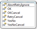
MessageBox::Show() can be called with one string argument: in that case, it will not have a header, and will have only the "OK” button. It is not a beautiful solution, is it?
The following example was already mentioned, now we will be able to interpret it:
System::Windows::Forms::DialogResult d;
d=MessageBox::Show("Are you sure that you would like to use the airbag?”, "Important security warning", MessageBoxButtons::YesNo);
if (d == System::Windows::Forms::DialogResult::No) e->Cancel=true;
The result of executing the code portion:
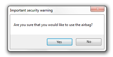
IV.2.22. Control used for timing: Timer

The Timer control makes it possible to run a code portion at given time intervals. It should be put under the form in the Designer, because it is not visible during execution. Its property named Interval contains the interval in milliseconds, and if the Enabled property is set to false, the timer can be disabled. If it is enabled and Interval contains a useful value (>=20 ms), the Timer executes its default event handler, the Tick. Progammers have to make sure that the code portion finish before the next event is occured (that is when time is out). The following code portion sets up the timer1 to run in every second:
timer1->Interval=1000; // every second timer1->Enabled=true; // go !
The programmed timer of the next code prints out the current time in seconds into the title of the form:
DateTime^ now=gcnew DateTime(); // variable of type time. now=now->Now; // what's the time? this->Text=Convert::ToString(now); // show in the title of the form.
This code portion can further be developed in order that it would play the cuckoo.wav sound file which is longer than one second: if (now->Minute==0) && (now->Second==0). If we think that the timer has already run enough times, int the Tick event handler the Enabled property can be set to false: at that case, the current event was the last.
IV.2.23. SerialPort

The SerialPort control makes possible the communication between a serial port of rs-232 standard and the peripherial devices connected to it (modem, SOC, microcontroller, Bluetooth device). The port has to be parameterized then opened. Then, textual information (Write, WriteLine, Read, ReadLine) and binary data (WriteByte, ReadByte) can be sent and received. It also has an event handler function: if data arrive, the DataReceived event is run. The following code portion checks all available serial ports, and searches the hardware named "iCorset" by sending a "?" character. If it is not found, it exits with an error message. In the case of virtual serial ports (USBs), the value of the BaudRate parameter can be anything.
array<String^>^ portnames;
bool there_is_a_controller=false;
int i;
portnames=Ports::SerialPort::GetPortNames();
i=0;
while (i<portnames->Length && (!there_is_a_controller))
{
if (serialPort1->IsOpen) serialPort1->Close();
serialPort1->PortName=portnames[i];
serialPort1->BaudRate=9600;
serialPort1->DataBits=8;
serialPort1->StopBits=Ports::StopBits::One;
serialPort1->Parity = Ports::Parity::None;
serialPort1->Handshake = Ports::Handshake::None;
serialPort1->RtsEnable = true;
serialPort1->DtrEnable = false;
serialPort1->ReadTimeout=200; // 0.2 s
serialPort1->NewLine="\r\n";
try {
serialPort1->Open();
serialPort1->DiscardInBuffer();// usb !
serialPort1->Write("?");
s=serialPort1->ReadLine();
serialPort1->Close();
} catch (Exception^ ex) {
s="Timeout";
}
if (s=="iCorset") there_is_a_controller=true;
i++;
}
if (! there_is_a_controller) {
MessageBox::Show("No iCorset Controller.",
"Error",MessageBoxButtons::OK);
Application::Exit();
}
IV.3. Text and binary files, data streams
The operative memory of a PC has a small size (as compared to the quantity of data to be stored) and forgets data easily: PC does not even have to be turned off, it is enough to exit a program, and the values of the variables stored in the memory are lost. That is why, even the first computers, manufactured after the ferrite-ring memory period, contained a data storage device that stored the software currently not in use or the data currently not used. The storage unit is the file which is a set of logically related data. It is the task of the operating system to connect a logical file to the physical organisation of the disk and to make them available for computer programs and to create and manage the file system. The programs using these files refer to them by their name. There are operations that process the content of the files and those that do not. For example, renaming or deleting a file does not require processing its content, it only requires its name. The name of the file may contain its path. If it does not contain it, the default path is the folder of the project during software development. When the .exe file, ready to be used, is run, the default folder is that of the .exe file.
IV.3.1. Preparing to handling files
Contrary to graphics or to controls, file handling namespace is not inserted in the form when a new project is created. This is the task of programmers to insert it at the beginning of the form1.h, where the other namespaces are:
using namespace System::IO;
Another thing to do is to decide what the file to be handled contains and what we would like to do with it:
Only deleting, renaming, copying it or checking whether it exists.
We would like to handle it by bytes (as a block containing bytes) if we are brave enough: virus detection, character encoding etc.
It is a binary file with fixed-length record structure.
If it is a text file with variable-length lines (Strings), and the lines end with line feed.
The file name can be given in two ways:
The file name is given in the code, therefore it is hard coded. If the file is only for the usage of programmer and it is always the same file, than this is a simple and rapid way of providing the name of the file.
Users can select the file by using OpenFileDialog or SaveFileDialog (see section Section IV.2.20, “Dialog windows helping file usage: OpenFileDialog, SaveFileDialog and FolderBrowserDialog”). In this case, the name of the file is stored in the FileName property of these dialog boxes.
IV.3.2. Methods of the File static class
bool File::Exists(String^ filename) It examines the existence of the file given in filename, if it exists, the output is true if not, it is false. By using it we can avoid some errors: opening a non-existing file, overwriting an important data file by mistake.
void File::Delete(String^ filename) It deletes the file given in filename. As opposed to current operating systems, deletion does not mean moving to a recycle bin but a real deletion.
void File::Move(String^ oldname, String^ newname) It renames the disk file named oldname to newname. If there are different paths in the filenames, the file moves into the other directory.
void File::Copy(String^ sourcefile, String^ targetfile) This method is similar to Move, except that the source file does not disappear but the file is duplicated. A new file is created on the disk, with the content of the source file.
FileStream^ File::Open(String^ filename, FileMode mode) Opening the given file. The FileStream^ does not get its value with gcnew but with this method. It does not have to be used for text files but for all the other files (containing bytes or binary files containing records) opening should be used. The values of mode:
FileMode::Appendwe go to the end of the text file and switch to write mode. If the file does not exist, a new file is created.FileMode::Createthis mode creates a new file. If the file already exists, it is overwritten. In the directory of the path, the current user should have a right for writing.FileMode::CreateNewthis mode also creates a new file but if the file already exists, we get an exception.FileMode::Openopening an existing file for reading/writing. This mode is generally used after creating the file, e.g. after using the FileOpenDialog.FileMode::OpenOrCreatewe open an existing file, if it does not exist, a file with the given name is created.FileMode::Truncatewe open an existing file and delete its content. The length of the file will be 0 byte.
IV.3.3. The FileStream reference class
If files are processed by bytes or they are binary, we need to create a FileStream^ object for the file. The class instance of FileStream is not created by gcnew but by File::Open(), so the physical disk file and FileStream are assigned to each other. With the help of FileStream the actual file pointer is accessable, and it can be moved. The measure unit of the position and the movement is byte; its data type is 64 bit integer so that it should manage files bigger than 2GB. Its most frequently used properties and methods:
Length: read-only property, the actual size of the file in bytes.
Name: the name of the disk file that we opened.
Position: writable/readable property, the current file position in bytes. The next writing operation will write into this position, the next reading will read from here.
Seek(how much, with regard to what) method for movng the file pointer. With regard to the Position property, it can be given how we understand movement: from the beginning of the file (
SeekOrigin::Begin), from the current position (SeekOrigin::Current), from the end of the file (SeekOrigin::End). This operation must be used also when we attach BinaryReader or BinaryWriter to FileStream since they do not have aSeek()method.int ReadByte(),WriteByte(unsigned char)methods for reading and writing data of one byte. Reading and writing happens in the current position. At the level of the operating system, file reading is carried out into a byte array; these functions are realized as reading an array with one element.int Read(array<unsigned char>, offset, count): a method for reading bytes into a byte array. The bytes will be placed from the array’s element with the index offset and the count is maximum number of bytes to read. Its return value is: how many bytes could be read.Write(array<unsigned char>,offset, count): a method for writing a block of bytes from a byte array. Writing begins at at the element with the index offset and it writes maximum count elements.Flush(void): clears buffers for this stream and causes any buffered data to be written to the file.Close(): closing FileStream. Files should be closed after use in order to avoid data loss and running out of resources.
IV.3.4. The BinaryReader reference class
If we want to read non-byte type binary data from a file, we use BinaryReader. In the BinaryReader ‘s constructor we give the opened FileStream handle as an argument. BinaryReader is created with a regular gcnew operator. It is important to note that BinaryReader is not able to open the disk file and to assign it to a FileStream. BinaryReader contains methods for the basic data types: ReadBool(), ReadChar(), ReadDouble(), ReadInt16(), ReadInt32(), ReadInt64(), ReadUInt16(), ReadString(), ReadSingle() etc. The file pointer is incremented with the length of the read data. BinaryReader also should be closed after use with the method Close() before closing the FileStream.
IV.3.5. The BinaryWriter reference class
If we want to write binary data into FileStream, we use BinaryWriter. It is created similarly to BinaryReader, with the operator gcnew. The difference is that Reader contained methods with a given return data type but Writer contains a method with a given parameter and without a return value, with a number of overloaded versions. The name of the method is Write and it can be used with several data types: from Bool to cli::Array^ in the order of complexity. The overview of binary file processing can be seen below:
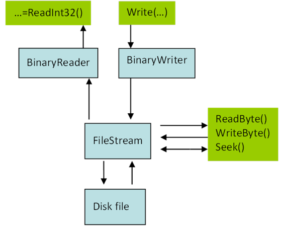
IV.3.6. Processing text files: the StreamReader and StreamWriter reference classes
Binary files that have been treated in the previous subsections are composed of fixed-length records. So a program can easily to calculate by a simple multiplication at which byte position the data to be searched for is and it can move the pointer to that position by the Seek() operation. For example if data are stored as 32-bit integers, each element occupies 4 bytes, the element having the index 10 (which actually is the 11th element) starts at the 10*4=40th byte position. In that case, as the file pointer can be moved anywhere, we speak about random access. Binary files can only be processed by a program which knows their record structure, which is in general, the program that created them.
Text files are composed of variable-length lines that are legible for human beings as well. In these files, characters are stored in ASCII, Unicode, UTF-8 etc. encoding, one line of a text file corresponds to the data type String^ of the compiler. Lines end with CR/LF (two characters) under DOS/Windows-based systems. Because of variable-length lines, text files can only be processed sequentially: reading the 10th line can be done by reading the first 9 lines and finally the requested 10th line. When the file is opened, it cannot be calculated at which byte the 10th line starts in the file, only after all preceding lines have been read.
Text files have an important role in realizing communication between different computer programs. Since they can be read for example in NotePad, humans can also modify their content. Text files are used, among other things, to save databases (in that case, a text file is called dump and it contains SQL statements that create the saved database on an empty system), to communicate with Excel (comma or tabulator separated files with CSV extension) and even e-mails are transferred as text files between incoming and outgoing e-mail servers. Measuring devices also create text files containing the measurement results. In these files, each line contains one measurement data in order that these data could be processed or visualized with any software (even with Excel) by a user carrying out the measurement.
Text files can be processed by reference variables of type StreamReader and StreamWriter classes. For that purpose, the gcnew operator should be used, and the name of the file should be specified in its constructor. A FileStream is not needed to be defined because StreamReader and StreamWriter use exclusively disk files; therefore they can create for themselves their own FileStream (BaseStream) with which programmers do not have to deal. The most frequently used method of StreamReader is ReadLine(), which reads the next line of the text file and its most frequently used property is EndOfStream, which becomes true accessing the end of the file. Attention: EndOfStream shows the state of the latest reading operation, ReadLine() returns a zero-length string at the end of the file, and the value of EndOfStream will be true. Thus, the ordinary pre-test loops can be used (while (! StreamReader->EndOfStream) …). One only has to examine if the length of the currently read line is greater than 0. The most frequently used method of StreamWriter is WriteLine(String), which writes the string passed as a parameter and `the newline character in the text file. Write(String) is the same but it does not write the newline character. The newline character(s) (CR,LF,CR/LF) can be set by the NewLine property.
The following code portion that does not function independently (i.e. without the helper functions and the initialisation parts) processes text files of CSV extension composed of semi-colon separated lines. The user is asked to select the file to be processed, the program reads the data line by line, calculates something from the read data and prints out the result at the end of the read line. After a file is processed, a total value is also calculated. Th program writes all outputs into a temporary file since the original text file is opened for reading. If data processing is done, the original file is deleted and the temporary file will receive the name of the original file. The result: the original text files will contain the results that have been calculated.
private: System::Void button1_Click(System::Object^ sender, System::EventArgs^ e) {
int m, credits, grade, creditsum = 0, gradesum = 0;
System::Windows::Forms::DialogResult dr;
String^ subject, ^line, ^outputstring = "";
openFileDialog1->FileName = "";
openFileDialog1->Filter = "CSV files (*.csv)|*.csv";
dr=openFileDialog1->ShowDialog(); // file open dialogbox, csv file
filename = openFileDialog1->FileName; // getting the file name
if (dr==System::Windows::Forms::DialogResult::OK ) // if it is not the Cancel button that was clicked
{
sr = gcnew StreamReader(filename); // open for reading
sw = gcnew StreamWriter(tmpname); // open the file for writing
while (!sr->EndOfStream) // always using a pre-test loop
{
line = sr->ReadLine(); // a line is read
if ((line->Substring(0,1) != csch) && (line->Length > 0))
// if it is not a separating character, it is processed
{
m = 0; // all lines are read from the first character
subject = newdata(line, m); // lines are split
credits = Convert::ToInt32(newdata(line, m)); // into 3 parts
grade = Convert::ToInt32(newdata(line, m));
// composing the output string
outputstring = outputstring + "subject:"+subject + " credits:" +
Convert::ToString(credits) +" grade:" +
Convert::ToString(grade) + "\n";
// and a weighted average is counted
creditsum = creditsum + credits;
gradesum = gradesum + credits * grade;
sw->WriteLine(line+csch+Convert::ToString(credits*grade));
} else { // is not processed but written back to the file.
sw->WriteLine(line);
} // if
} // while
sr->Close(); // do not forget to close the file
wa = (double) gradesum / creditsum; // otherwise the result is integer
// the previous line contained \n at its end, the result is written in a new line
outputstring = outputstring + "weighted average:" + Convert::ToString(sa);
label1->Text = outputstring;
sw->WriteLine(csch + "weighted average"+ csch + Convert::ToString(wa));
sw->Close(); // output file is also closed,
File::Delete(filename); // the old data file is deleted
// and the temporary file is renamed to the original data file.
File::Move(tmpname, filename);
}
}
IV.3.7. The MemoryStream reference class
One can also create sequential files, composed of bytes that are not stored on a disk but in the memory. A great advantage of streams created in the memory is the speed (a memory is at least two times faster than a storage device), its disadvantage is its smaller size and that its content is lost if the program is exited. MemoryStream has the same methods as FileStream: it reads/writes a byte or an array of bytes. It can be created by the gcnew operator. The maximal size of a MemoryStream can be set in the parameter of the constructor. If no parameter is given, MemoryStream will allocate memory dynamically for writing. Using that class has two advantages as compared to arrays: on one hand, automatic allocation and on the other hand, a MemoryStream can easily be transformed into a FileStream if memory runs out by using File::Open() instead of gcnew.
IV.4. The GDI+
The GDI Graphics Device Interface is a device independent (printer, screen) module of Windows systems used to develop and visualize 2D graphics (gdi.dll, gdi32.dll). The GDI+ is the improved version of this module that is also 2D and was introduced first in Windows XP and Windows Server 2003 operating systems (GdiPlus.dll). Newer Windows systems ensure the compatibility with programs developed with older versions, however, programmers can also use the optimized, inherited and new features of GDI+.
IV.4.1. The usage of GDI+
GDI+ was developed with object-oriented approach, that is, a 32/64 bit graphical programming interface which offers classes of C++ to draw in managed (.NET) as well as non-managed (native) programs. The GDI is not directly connected to the graphical hardware but to its driver. The GDI is capable of visualizing 2D vector-graphic illustrations, handling images and displaying textual information of publications in a flexible manner:
2D vector graphics: when making drawings, lines, curves and shapes bounded by these are defined by points given in coordinate system, and can be drawn with pens and painted with brushes..
Storing and displaying images: besides the flexible image storing and manipulating features, it offers the possibility to read and save a variety of image formats (BMP, GIF, JPEG, Exif, PNG, TIFF, ICON, WMF, EMFll).
Displaying texts: it is the task of GDI+ to visualize plenty of fonts on the screen as well as on the printer device.
The basic functions of GDI+ are contained in the System::Drawing namespace. Further options of 2D drawing can be reached using the elements of the
System::Drawing::Drawing2D
namespace.
The
System::Drawing::Imaging
namespace contains classes for handling images in an advanced level, whereas the
System::Drawing::Text
namespace ensures the special options of textual visualization
[4.1.]
.
IV.4.2. Drawing features of GDI
In order to use the basic functions of GDI+ in our program we have to use the System::Drawing namespace. (So that it can be reached the System.Drawing DLL file should be listed among the references Project / Properties / References: ).
using namespace System::Drawing;
The System::Drawing namespace contains the classes required for drawing (Figure IV.27, “The classes of GDI+”). It is worth to highlight the Graphics class which is modelling the drawing area like it was a drawing paper. In order to draw on the drawing paper some data structures are required that are defined in the System::Drawing namespace. We can define on the drawing paper which coordinate system to use. The color model used by GDI+ is the alfa-r-g-b model (the Color structure), that is, colors can be mixed not only with the primary colors of red, green and blue but the level of transparency of the color can be set by the alfa parameter.
The integer type x and y coordinates of points can be stored in the Point structure, in case of real (float) coordinates PointF can be used. Similarly to the points the Rectangle and RectangleF structures can be used to store and access the corners of rectangles in a variety of ways. The Size and SizeF structures can be used to store the vertical and horizontal size of shapes.
Real drawing tools are modeled by classes. Our basic drawing tool is the pen (Pen class that cannot be inherited). We can set its color, width and pattern. The tool for painting planar shapes is the brush (Brush parent class). The derived classes of Brush are the SolidBrush that are modeling a brush dipped into a single color and the TextureBrush that leaves marks of a bitmap pattern. The HatchBrush paints a hatched pattern, whereas the LinearGradientBrush and PathGradientBrush leaves gradient marks. In order to use these latest classes the
System::Drawing::Drawing2D
namespace is required, too. The derived brushes cannot be inherited further. The Image abstract class has properties and member functions used to store and handle bitmaps and metafiles. The Font class contains various character forms, that is fonts. The FontFamily is the model of font families. Neither the Font nor the FontFamily classes cannot be inherited further. The Region class (cannot be inherited) is modelling an area of the graphic tool bounded by the sides of rectangles and paths. The Icon class serves to handle Windows icons (small size bitmaps).
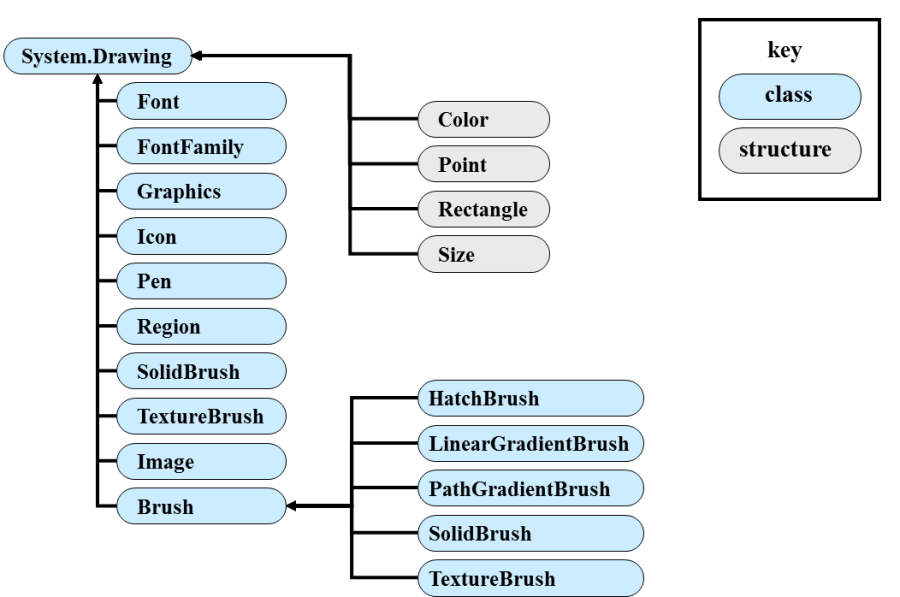
IV.4.3. The Graphics class
Before getting familiar with the Graphics class, let’s have a few words about the Paint event of the controls. The graphic objects appearing in the windows have to be often redrawn for example when being repainted. This happens in a way that the Windows automatically invalidates the area that we would like to repaint and calls the handler function of the objects’ Paint event. In case we would like to refresh our drawing on top of the objects popup from the hiding, then we have to place the drawing methods of the Graphic class in the handler functions of the Paint event. The event handler of the Paint event has a PaintEventArgs type reference parameter that are defined by Windows when calling
[4.2.]
.
private: System::Void Form1_Paint(
System::Object^ sender,
System::Windows::Forms::PaintEventArgs^ e){ }
The PaintEventArgs class have two properties, the Rectangle type ClipRectangle that contains data of the area that we would like to repaint and the Graphics type read-only Graphics that identifies the drawing paper as a drawing tool when repainting.
Later, we will show in more details how to create Pen type pen for drawing with the gcnew operator and how to define its color by the constructor argument using the Color::Red constant of the System::Drawing namespace. Once we have our pen, then the Line() method of the Graphics class can draw lines with it (Figure IV.28, “The drawn line automatically appears after every resizing activity.”).
private: System::Void Form1_Paint(System::Object^ sender,
System::Windows::Forms::PaintEventArgs^ e){
Pen ^ p= gcnew Pen(Color::Red);
e->Graphics->DrawLine(p,10,10,100,100);
}
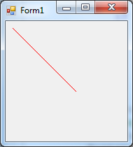
We can also initiate the repainting of windows and controls anywhere in the program. The Invalidate(), Invalidate(Rectangle) and Invalidate(Region) methods of the Control class invalidate the entire window / control or the selected area of them and activate the Paint event. The Refresh() method of the Control class invalidates the area of the window / control and initiates the repainting immediately.
We can draw on the window anywhere from the program if we create an instance of the drawing paper from the Graphics class with the CreateGraphics() method of the control / window. This time, however, the line drawn with the blue pen appears only once and will not be redrawn after hiding.
Pen ^ p= gcnew Pen(Color::Blue);
Graphics ^ g=this->CreateGraphics();
g->DrawLine(p,100,10,10,100);
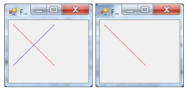
We can clear the given drawing paper with the defined background color by the
Clear(Color & Color);
method of the Graphics class.
IV.4.4. Coordinate systems
With the help of GDI+ we can think in three coordinate systems. We can create our model that we like to draw in 2D in the world coordinate system. It is useful to use such mapping that we could give these world coordinates to the drawing methods. Since the drawing methods of the Graphics class are able to receive the integer numbers (int) and floatingpoint real numbers (float) as parameters, that is why it is useful to store the world coordinates as int or float type too. We have to do ourselves the projection of 3D world to plane. The drawing paper modeled by the Graphics type reference uses the page coordinate system and it can be a form, an image storage or even a printer. It is the device coordinate system that a given tool uses (for example the left upper corner of the screen is the origin and the pixels are the units). Thus when drawing two mapping should happen:
world_coordinate → page_coordinate → device_coordinate
The first mapping have to be done by ourselves. We have more choices to obtain this. Spatial points can be projected to the plane in two ways, with parallel or central projection rays.
Projection with parallel ray is called axonometry. We can set up the mathematical model of projection by drawing the parallely projected image of x-y-z three-dimensional coordinate system to the planar sheet of the ξ-η coordinate system, assuming that the image of the three-dimensional coordinate system’s origin is the origin of the planar coordinate system. The image of x-y-z three-dimensional coordinate system appears with dashed lines in the ξ-η coordinate system drawn with solid lines (Figure IV.30, “General axonometry”). According to Figure IV.30, “General axonometry” let’s mark the angle between ξ- and x-axes with α, the angle between ξ- and y-axes with β and the angle between η- and z-axes with γ! As the x-y-z coordinate axes are not parallel with the plane ξ-η, the image of coordinate units projected to the planar coordinate system seems to be shorter. The x-direction seems to be q x (≤1) long, the y-direction unit q y (≤1) and the z-direction unit q z (≤1) long.
Therefore, if we are looking for the planar, mapped coordinates (ξ,η) of a point with coordinates (x,y,z), then the pair of functions (f ξ , f η ) implements the mapping according to (IV.4.1).
|
|
(IV.4.1) |

Mapping can be described simply, if we consider that starting from the origin we are moving units x, y and z parallel to the images of the axes according to the shortenings, thus getting to the image (ξ, η) of point (x, y, z) (Figure IV.30, “General axonometry”). It follows that summarizing the projections of ξ and η with the red arrow, we get the coordinates as follows (IV.4.2).
|
|
(IV.4.2) |

A special type of axonometry is the isometric axonometry, when there is a 120° angle between the projections of x-y-z axes, the projection of z-axis coincides with η-axis (α=30, β=30, γ=0) and the shortenings are q x =q y =q z =1 (Figure IV.31, “Isometric axonometry”).
Another widely used axonometry is the Cavalier or military axonometry, where the horizontal y- axis coincides with the ξ-axis, the vertical z-axis coincides with the η-axis and there is a 135° angle between the projection of the x-axis and the other two axes (α=45, β=0, γ=0). The shortenings are q x =0,5, q y =q z =1.
By default, the origin of the sheet’s 2D coordinate system – in case of form – is in the top left corner of the form’s active area, the x-axis is pointing to the right, while the y-axis is pointing down and the units are pixels in both axes (Figure IV.33, “The default coordinate-system on form”).
Therefore, until any further actions are taken, the arguments of the already-known DrawLine() method of the Graphics class are values in this coordinate system.
As an example, let’s create the function producing the mapping of Cavalier axonometry. The input parameters of this function are the spatial coordinates (x, y, z), by substituting the constants of the Cavalier axonometry (IV.4.2) the function returns a PointF type sheet point.
PointF Cavalier(float x, float y, float z) {
float X = 0;
float Y = 0;
X=(-x*(float)Math::Sqrt(2)/2/2+y);
Y=(-x*(float)Math::Sqrt(2)/2/2+z);
return PointF(X, Y);
}
As an example, using the Cavalier() function and the DrawLine() method of the Graphics class, let’s draw in the Paint event handler a 100 units sided cube centred at point (250,250,250) illustrated in axonometry.
private: System::Void Form1_Paint(System::Object^ sender,
System::Windows::Forms::PaintEventArgs^ e) {
// the centre and the half side
float ox=250;
float oy=250;
float oz=250;
float d=50;
// The red pen
Pen ^p=gcnew Pen(Color::Red);
// The upper side
e->Graphics->DrawLine(p,Cavalier(ox-d,oy-d,oz-d),
Cavalier(ox+d,oy-d,oz-d));
e->Graphics->DrawLine(p,Cavalier(ox+d,oy-d,oz-d),
Cavalier(ox+d,oy+d,oz-d));
e->Graphics->DrawLine(p,Cavalier(ox+d,oy+d,oz-d),
Cavalier(ox-d,oy+d,oz-d));
e->Graphics->DrawLine(p,Cavalier(ox-d,oy+d,oz-d),
Cavalier(ox-d,oy-d,oz-d));
// The lower side
e->Graphics->DrawLine(p,Cavalier(ox-d,oy-d,oz+d),
Cavalier(ox+d,oy-d,oz+d));
e->Graphics->DrawLine(p,Cavalier(ox+d,oy-d,oz+d),
Cavalier(ox+d,oy+d,oz+d));
e->Graphics->DrawLine(p,Cavalier(ox+d,oy+d,oz+d),
Cavalier(ox-d,oy+d,oz+d));
e->Graphics->DrawLine(p,Cavalier(ox-d,oy+d,oz+d),
Cavalier(ox-d,oy-d,oz+d));
// The lateral edges
e->Graphics->DrawLine(p,Cavalier(ox-d,oy-d,oz-d),
Cavalier(ox-d,oy-d,oz+d));
e->Graphics->DrawLine(p,Cavalier(ox+d,oy-d,oz-d),
Cavalier(ox+d,oy-d,oz+d));
e->Graphics->DrawLine(p,Cavalier(ox+d,oy+d,oz-d),
Cavalier(ox+d,oy+d,oz+d));
e->Graphics->DrawLine(p,Cavalier(ox-d,oy+d,oz-d),
Cavalier(ox-d,oy+d,oz+d));
}
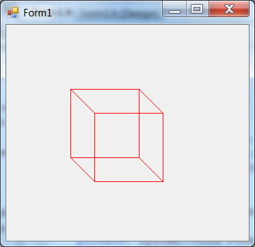
It is clearly shown in Figure IV.34, “Cube in axonometry” that axonometric mapping keeps distance in the given coordinate direction. Therefore, the back edge of the cube seems to have the same length as the front edge. However, using our eyes, we do not get this very same image. Our eyes perform central projection.
Central projection projects spatial points to the picture plane with the help of rays arriving at a certain point. In order to get the simple formulas of central projection, let’s suppose that we project the points of the spatial x-y-z coordinate system to the picture plane S parallel with x-y plane. Let’s mark the origin of the spatial x-y-z coordinate system with C. C will be the centre of projection. The orogin of ξ-η coordinate system in plane S should be O, and let it to be of d distance from C on the z-axis of the spatial coordinate system. The axes of ξ-η coordinate system of plane S are parallel with x- and y-axes (Figure IV.35, “Central projection”). Let’s find the mapping of the central projection corresponding to (IV.4.1).
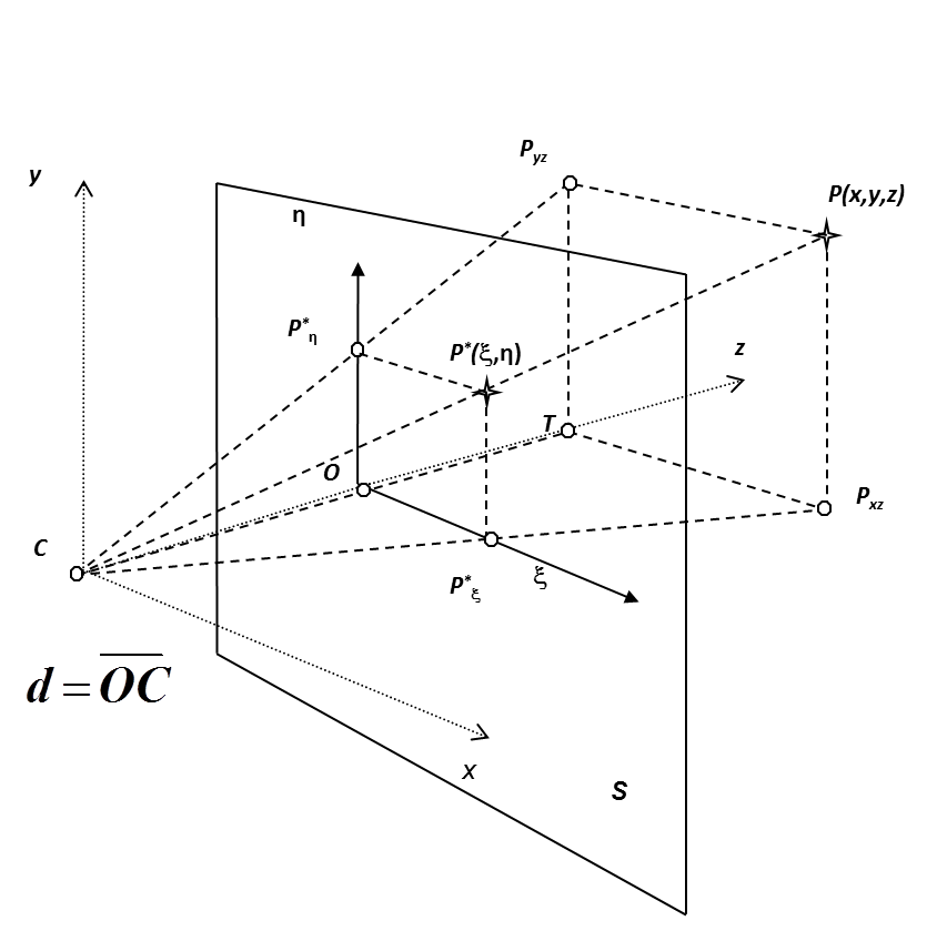
As shown in the graphic, let the distance of the origin and centre be d. Let x, y, z be the coordinates of a spatial point P and let the projection of this point be P * in the plane with coordinates ξ, η. The projection of point P to x-z plane is Pxz (of which distance from z-axis is coordinate x exactly), to y-z plane it is P yz (of which distance from z axis is coordinate y exactly). The projection of P xz in plane S is P * ξ , of which distance from the origin of the planar coordinate-system is coordinate ξ exactly, the projection of P yz in plane S is P * η of which distance from the zero point of the planar coordinate-system is coordinate η exactly. As triangle COP * ξ is similar to triangle CTP xz , therefore
|
|
(IV.4.3) |

that is
|
|
(IV.4.4) |

Similarly, in plane yz triangle CTP yz is similar to triangle COP η , therefore
|
|
(IV.4.5) |

that is
|
|
(IV.4.6) |

With this we generated (IV.4.1) mapping, as after rearranging we get
|
|
(IV.4.7) |


The problem with formulas in (IV.4.7) is that the mapping is not linear. We can make it linear by increasing the number of dimensions (from two to three), and we introduce homogeneous coordinates. Let’s have a four-dimensional point [x, y, z, 1] instead of the spatial point [x, y, z]. That is we are thinking in the w=1 three-dimensional subspace within the four-dimensional space of [x, y, z, w]. In this space the mapping of (IV.4.7) is
|
|
(IV.4.8) |

which is linear since it can be rewritten to form (IV.4.9).
|
|
(IV.4.9) |

As an example, let’s make the Perspective function performing the mapping of central projection. Input parameters are spatial coordinates (x, y, z). By giving the focal length d and using formulas (IV.4.4, IV.4.6), the function gives a PointF type sheet point.
PointF Perspective(float d, float x, float y, float z) {
float X = 0;
float Y = 0;
X = d * x / z;
Y = d * y / z;
return PointF(X, Y);
}
As an example, using the Perspective() function and the well-known DrawLine() method of the Graphics class, let’s draw in the Paint event handler a 100 units sided cube centred at point (150,150,150) illustrated in perspectiveaxonometry with f=150, f=450 and f=1050 focal lengths (Figure IV.36, “The perspective views of the cube”).
private: System::Void Form1_Paint(
System::Object^ sender,
System::Windows::Forms::PaintEventArgs^ e) {
// the centre and the half side
float ox=150;
float oy=150;
float oz=150;
float d=50;
float f=350;
// The red pen
Pen ^p=gcnew Pen(Color::Red);
// The upper side
e->Graphics->DrawLine(p,Perspective(f,ox-d,oy-d,oz-d),
Perspective(f,ox+d,oy-d,oz-d));
e->Graphics->DrawLine(p,Perspective(f,ox+d,oy-d,oz-d),
Perspective(f,ox+d,oy+d,oz-d));
e->Graphics->DrawLine(p,Perspective(f,ox+d,oy+d,oz-d),
Perspective(f,ox-d,oy+d,oz-d));
e->Graphics->DrawLine(p,Perspective(f,ox-d,oy+d,oz-d),
Perspective(f,ox-d,oy-d,oz-d));
// The lower side
e->Graphics->DrawLine(p,Perspective(f,ox-d,oy-d,oz+d),
Perspective(f,ox+d,oy-d,oz+d));
e->Graphics->DrawLine(p,Perspective(f,ox+d,oy-d,oz+d),
Perspective(f,ox+d,oy+d,oz+d));
e->Graphics->DrawLine(p,Perspective(f,ox+d,oy+d,oz+d),
Perspective(f,ox-d,oy+d,oz+d));
e->Graphics->DrawLine(p,Perspective(f,ox-d,oy+d,oz+d),
Perspective(f,ox-d,oy-d,oz+d));
// The lateral edges
e->Graphics->DrawLine(p,Perspective(f,ox-d,oy-d,oz-d),
Perspective(f,ox-d,oy-d,oz+d));
e->Graphics->DrawLine(p,Perspective(f,ox+d,oy-d,oz-d),
Perspective(f,ox+d,oy-d,oz+d));
e->Graphics->DrawLine(p,Perspective(f,ox+d,oy+d,oz-d),
Perspective(f,ox+d,oy+d,oz+d));
e->Graphics->DrawLine(p,Perspective(f,ox-d,oy+d,oz-d),
Perspective(f,ox-d,oy+d,oz+d));
}
We can see the effect of focal length. Focal length-change behaves exactly the same as the objective of cameras. In case of small focal length there is a large viewing angle and strong perspective, in case of large focal length there is a small viewing angle and weak perspective.
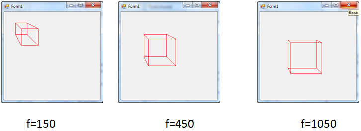
In the examples above we ensured that spatial coordinates are always projected to the plane, and we chose the centre and size of the cube in a way that it surely gets to the picture. The units of the cube’s data can be given either in mm, m or km. By drawing the cube to the form, the centres and the length of the edges were all given in pixels. However, by this we implicitly performed a zoon in/zoom out (mm->pixel, m->pixel or km->pixel). Based on the window sizes and the geometry to be displayed this should always be defined (Window-Viewport transformation
[4.3.]
). In GDI+ we can use the Transform property of the Graphics class to create coordinate transformation, thereby a Window-Viewport transformation can also be easily performed.
IV.4.5. Coordinate transformation
As we have seen the origin of the page coordinate system is the top left corner of the active area of the window, the x-axis points to the right, the y-axis points down and the units are pixels (Figure IV.33, “The default coordinate-system on form”). The Transform property of the Graphics class is a reference pointing to an instance of the Matrix class. The Matrix class is defined on the System::Drawing::Drawing2D; namespace.
The Matrix class is the model of a transformation matrix of the 2D plane with homogeneous coordinates that contain 3x3 elements and its third column [0,0,1]T. The m
11
, m
12
, m
21
, m
22
mean the rotation and the scaling along the axes of the coordinate transformation, whereas d
x
, d
y
mean the translation (IV.4.10).
|
|
(IV.4.10) |

Transformation matrixes implement geometric transformations
[4.4.]
. Processing the geometric transformations one after the other results in one single geometric transformation. The transformation matrix of this is the first transformation matrix multiplied by the second transformation matrix from the left. Applying the geometric transformation matrixes one after the other is a non-commutative operation similarly to multiplying matrixes which is also non- commutative. We have to pay attention to this when assigning the Transform property. For defining the transformation we can use the methods of the Matrix class.
We can create a transformation matrix instance with the constructors of the Mátrix class. The
Matrix()
constructor activated without a parameter creates a three dimensional identity matrix. For example if we create an E identity matrix and we assign it to the Graphics->Trasform property, it will keep the coordinate system shown on Figure IV.33, “The default coordinate-system on form”.
private: System::Void Form1_Paint(System::Object^ sender,
System::Windows::Forms::PaintEventArgs^ e) {
Matrix ^ E=Matrix();
e->Graphics->Transform=E;
Pen ^ p= gcnew Pen(Color::Red);
e->Graphics->DrawLine(p,10,10,100,100);
}
We can achieve the same result with the void type Reset() method of the Matrix class:
Matrix ^ E=Matrix();
E->Reset();
We can define any transformation (that is linear in homogeneous coordinates) if we use one of the parametric constructors. As a definition of the transformation we can distort a rectangle into a parallelogram while moving it at the same time (Figure IV.37, “Setting the distortion”). In order to achieve this we can create the transformation with the following parametric constructor:
Matrix(Rectangle rect, array<Point>^ points)
The constructor creates such a geometric transformation that distorts the rect rectangle set as the parameter to a parallelogram (Figure IV.37, “Setting the distortion”). The points array contains three points. Respectively the first element is the upper left corner point of the parallelogram (ul), the second element is the upper right corner point (ur) and the lower left corner point is the third one (ll) (the place of the fourth point will be derived).
The DrawRectangle() method of the Graphics class draws a rectangle on the form with setting the pen, the starting coordinates, the width and the height. In the next example we will draw a rectangle of (10,10) starting points, 100 width and 100 height size values in red. With setting a transformation we modified the rectangle in a way that it was placed into (20,20) starting points, its height to be 200 and to be inclined 45 degrees. After this we drew the same rectangle in blue, and we can see the translation, the scaling and the shearing were applied.
private: System::Void Form1_Paint(System::Object^ sender,
System::Windows::Forms::PaintEventArgs^ e) {
Pen ^ pen= gcnew Pen(Color::Red);
e->Graphics->DrawRectangle(pen,10,10,100,100);
array< PointF >^ p = {PointF(120,220), PointF(220,220),
PointF(20,20)};
Matrix ^ m = gcnew Matrix(RectangleF(10,10,100,100),p);
e->Graphics->Transform=m;
pen= gcnew Pen(Color::Blue);
e->Graphics->DrawRectangle(pen,10,10,100,100);
}
The transformation matrix can be set by elements (formula IV.4.7) as well using the other parametric constructor:
Matrix(float m11, float m12, float m21, float m22, float dx, float dy);
The next example uses a translaion (10, 10), double scaling in x-direction and 1.5x scaling in y-direction:
private: System::Void Form1_Paint(System::Object^ sender,
System::Windows::Forms::PaintEventArgs^ e) {
Pen ^ pen= gcnew Pen(Color::Red);
e->Graphics->DrawRectangle(pen,0,0,100,100);
Matrix ^ m = gcnew Matrix(2,0,0,1.5,50,50);
e->Graphics->Transform=m;
pen= gcnew Pen(Color::Blue);
e->Graphics->DrawRectangle(pen,0,0,100,100);
}
Of course we can access the elements of the matrix using the (Array<float> type) Elements read only property of the Matrix class.
Fortunately we can create a transformation not only with setting the coordinates in the matrix but with the transformational methods of the Matrix class as well. We can apply the transformational functions to the instaces of the Matrix class as we multiplied the matrix of the current instance from the right or from the left by the matrix of the transformational method. The MatrixOrder type enumeration helps to control this and its members are MatrixOrder::Prepend (0, from the right) and MatrixOrder::Append (1, from the left).
We can directly multiply the instance of the class that contains the matrix by the given Matrix transformation matrix:
Multiply(Matrix matrix [,MatrixOrder order])
The square bracket means that it is not mandatory to set the MatrixOrder type order parameter. The default value of the order parameter is MatrixOrder::Prepend. We skip the explanation of the square brackets in case of the next methods.
We can define a translation and apply it on the matrix instance with the method:
Translate(float offsetX, float offsetY
[,MatrixOrder order]);
We can perform rotation transformation around the origin of the coordinate system with angle alfa
Rotate(float alfa [, MatrixOrder order])
or around a given point with alfa angle (set in degrees!);
RotateAt(float alfa, PointF point [,MatrixOrder order]);
Both methods are void methods.
The next example rotates a line around the midpoint of the form. In order to achieve this we have to know that the Size tpye ClientSize property of the form contains the dimensions of the client area.
private: System::Void Form1_Paint(System::Object^ sender,
System::Windows::Forms::PaintEventArgs^ e) {
Matrix ^ m = gcnew Matrix();
Pen ^ p = gcnew Pen(Color::Red);
float x=this->ClientSize.Width/2;
float y=this->ClientSize.Width/2;
for (int i=0; i<360; i+=5) {
m->Reset();
m->Translate(x,y);
m->Rotate(i);
e->Graphics->Transform=m;
e->Graphics->DrawLine(p,0.0F,0.0F,
(float)Math::Min(this->ClientSize.Width/2,
this->ClientSize.Height/2),0.0F);
}
}
We can apply scaling (scaleX, scaleY) along the coordinate axes with a similar function:
Scale(float scaleX, float scaleY[, MatrixOrder order]);
Shearing along one of the coordinate direction means that the axis remains in place and as we move away from the axis parallel translation of the points along the fixed axis is proportional with the distance from the axis.
The transformation matrix contaning homogeneous coordinate of the shearing is:
|
|
(IV.4.11) |

We also have a function to define the shearing, where we can set the shearing coordinates of the matrix:
Shear(float mX, float mY, [, MatrixOrder order]);
In the next example we translate and shear a rectangle in both directions:
private: System::Void Form1_Paint(System::Object^ sender,
System::Windows::Forms::PaintEventArgs^ e) {
Pen ^ pen= gcnew Pen(Color::Red);
e->Graphics->DrawRectangle(pen,0,0,100,100);
Matrix ^m=gcnew Matrix();
m->Translate(10,10);
m->Shear(2,1.5);
e->Graphics->Transform=m;
pen= gcnew Pen(Color::Blue);
e->Graphics->DrawRectangle(pen,0,0,100,100);
}
We can calculate the inverse of the transformation matrix with the void tpye method of the Matrix class:
Invert();
If we do not want to use the Transform property of the Graphics class then we can use directly the following methods of the Graphics class that directly modify the Transform property:
ResetTransform()
MultiplyTransform(Matrix m, [, MatrixOrder order]);
RotateTransform(float szog , [, MatrixOrder order])
ScaleTransform(float sx, float sy[, MatrixOrder order])
TranslateTransform Method(float dx, float dy
[, MatrixOrder order])
The Sheet transformation that maps sheets to a device can use the PageUnit and PageScale properties of the Graphics class in order to define the mapping. The PageUnit property can take a value of the System::Drawing::GraphicsUnit enumeration (UnitPixel=2, UnitInch=4, UnitMillimeter=6…).
For the example we set millimeter as a sheet unit. If the length of side of the square is 20 mm, then it will be also around 20 mm on the screen. If we set the float type PageScale property of the Graphics class then it will set our scaling on the sheet. For example if PageScale = 0.5 then the 20 mm sided square will become 10 mm (Figure IV.39, “Trasnlating and scaling with a matrix”).
private: System::Void Form1_Paint(System::Object^ sender,
System::Windows::Forms::PaintEventArgs^ e) {
e->Graphics->PageUnit=GraphicsUnit::Millimeter;
Pen ^ pen= gcnew Pen(Color::Red);
e->Graphics->DrawRectangle(pen,10,10,30,30);
e->Graphics->PageScale=0.5;
pen= gcnew Pen(Color::Blue);
e->Graphics->DrawRectangle(pen,10,10,30,30);
}
The GDI+ receives the screen resolution information from the driver and it can set the data of the mapping from here. The DpiX and DpiY read only properties contain the dot/inch resolution for the given device.
IV.4.6. Color handling of GDI+ (Color)
We use the Color structure to store GDI+ colors. This is nothing more than a 32-bit integer which each byte has a meaning (compared to traditional GDI colors where only 24 bits from the 32 coded colors). The 32-bit information is called ARGB color, the most significant byte (Alpha) shows the transparency, the rest 24 bits code the intensity of the GDI related Red, Green and Blue color components. (Alpha=0 is fully transparent, 255 is not transparent, the values for the color componenets indicate the intensity of them.) We can create a color structure with the FromArgb() method of the System::Drawing::Color structure. Calling the overloaded versions of the FromArgb() we can pass 3 integer (r, g and b) or 4 integer (a, r, g and b) arguments. In addition we can use more predefined normal colors Color::Red, Color::Blue etc. and system colors SystemColors::Control, SystemColors::ControlText etc.
The well-known application used to set the background color of the window shows well the usage/applicability of RGB colors. The background color of the window can be only an RGB color. Let us put three vertical sliders (scrollbars) to the form. The names (Name) should be red, green and blue respectively.
Let’s set their upper limit to 255 (not caring about the fact that the slider cannot go up to 255). The Scroll event of each should be the evet handler of the red, as it is apparent in the code generated by the Designer.
//
// red
//
this->red->Location = System::Drawing::Point(68, 30);
this->red->Maximum = 255;
this->red->Name = L"red";
this->red->Size = System::Drawing::Size(48, 247);
this->red->TabIndex = 0;
this->red->Scroll += gcnew
System::Windows::Forms::ScrollEventHandler(
this, &Form1::red_Scroll);
//
// green
//
this->green->Location = System::Drawing::Point(187, 30);
this->green ->Maximum = 255;
this->green ->Name = L"green";
this->green ->Size = System::Drawing::Size(48, 247);
this->green ld->TabIndex = 1;
this->green ->Scroll += gcnew
System::Windows::Forms::ScrollEventHandler(
this, &Form1::red_Scroll);
//
// blue
//
this->blue->Location = System::Drawing::Point(303, 30);
this->blue->Maximum = 255;
this->blue->Name = L"blue";
this->blue->Size = System::Drawing::Size(48, 247);
this->blue->TabIndex = 2;
this->blue->Scroll += gcnew
System::Windows::Forms::ScrollEventHandler(
this, &Form1::red_Scroll);
The event handler of the red slider’s Scroll event uses the position of all the three sliders to set the background color (Value property):
private: System::Void red_Scroll(System::Object^ sender,
System::Windows::Forms::ScrollEventArgs^ e) {
this->BackColor = Color::FromArgb(
red->Value, green->Value, blue->Value);
}
We will get familiar with the usage of transparent colors with the pen and brush drawing tools. The read only property of the Color structure, that is, the R, G and B (Byte type) properties contain the color components.
Byte r = this->BackColor.R;
IV.4.7. Geometric data (Point, Size, Rectangle, GraphicsPath)
We can create geometric objects with the Point, PointF and the Rectangle, RectangleF structures, and we can store the dimensions of rectangles within the Size, SizeF structures. The closing F letter refers to the float type of the structure’s data members. If the letter F is missing, then the data members are of type int.
IV.4.7.1. Storing dimensions
We can create Size structures with the
Size(Int32,Int32)
Size(Point)
SizeF(float,float)
SizeF(PointF)
constructors. The Height and Width properties of the Size and the SizeF structures (int and float) contain the height and width values of rectangles. The logical type IsEmpty property informs about if both size properties are set to 0 (true) or not (false).
With the size data we can perform operations with the methods of Size(F) structures. The Add() method adds the Width and Height values of Size type parameters, whereas Subtract() subtracts them.
static Size Add(Size sz1, Size sz2);
static Size Subtract(Size sz1, Size sz2);
We can compare the equality of two size structures with
bool Equals(Object^ obj)
According to the above methods there are defined the overloaded +, - and == operators of the Size(F) structures.
SizeF type values are rounded up to Size type with the Ceiling(), whereas the Round() method rounds in the usual way.
static Size Ceiling(SizeF value);
static Size Round(SizeF value);
The ToString() method converts the Size(F) structure to the form of a {Width=xxx, Height=yyy} string.
It is important to note that since the forms have a Size property, the Size type structure can be used only by defining the namespace. The following example writes the size values of the generated Size to the header of the form:
System::Drawing::Size ^ x= gcnew System::Drawing::Size(100,100); this->Text=x->ToString();
IV.4.7.2. Storing planar points
The Point, PointF structures are very similar to the Size structures with aspect their purpose, however they are defined to store point coordinates. Points can be created with the foolowing contructors:
Point(int dw);
Point(Size sz);
Point(int x, int y);
PointF(float x, float y);
In the first case the coordinate x is defined by the lower 16 bits of the parameter and the coordinate y is defined by the upper. In the second case x is defined by the Width property of the Size type parameter and y is defined by the Height property. The basic properties of the point structures are the X, Y coordinate values and the IsEmpty analysis.
We can perform point operations with the methods of the Point(F) structures. The Add() method adds the Width and Height values of the Size structure that was received also as a parameter, whereas Subtract() subtracts them.
static Point Add(Point pt, Size sz);
static Size Subtract(Point pt, Size sz);
We can investigate the equality of two Point type structures with the Equals() method:
virtual bool Equals(Object^ obj) override;
According to the above methods there are defined the overloaded +, - and == operators of the Point(F) structures.
A PointF type value rounds up to Point type the Ceiling() method, whereas the Round() method rounds in the usual way.
static Size Ceiling(SizeF value);
static Size Round(SizeF value);
The ToString() method converts the Point(F) structures to the form of a {X=xxx, Y=yyy} string.
IV.4.7.3. Storing planar rectangles
The Rectangle and the RectangleF structures are used to store the data of rectangles. Rectangles can be created with the
Rectangle(Point pt, Size sz);
Rectangle(Int32 x, Int32 y, Int32 width, Int32 height);
RectangleF (PointF pt, SizeF sz);
RectangleF(Single x, Single y, Single width, Single height);
constructors. The X, Y, the Left, Top and the Location properties of the Rectangle(F) structure contain the coordinates of the upper-left corner. The Height, Width and Size are the latitude and elevation dimensions of the rectangles, the Right and Bottom properties are the coordinates of the lower-right corner. The IsEmpty informs about whether our rectangle is real or not. The Empty is a rectangle with undefined data:
Rectagle Empty;
Empty.X=12;
We can create a rectangle (Rectangle, RectangleF) with the specified upper-left and lower-right corner coordinates:
static Rectangle FromLTRB(int left,int top,
int right,int bottom);
static RectangleF FromLTRB(float left, float top,
float right, float bottom)
The Rectangle structure offers a lot of methods to be used. From the RectanleF structure creates a Rectangle structure by rounding up the Ceiling() method, by normal rounding the Round() method and by cutting the decimal part the Truncate() method.
We can decide if the rectangle contains a point or a rectangle. With the methods of the Rectangle structure:
bool Contains(Point p);
bool Contains(Rectangle r);
bool Contains(int x, int y);
or the methods of the RectangleF structure:
bool Contains(PointF p);
bool Contains(RectangleF r);
bool Contains(single x, single y);
We can increase the area of the current Rectangle(F) by specifying the width and height data:
void Inflate(Size size);
void Inflate(SizeF size);
void Inflate(int width, int height);
void Inflate(single width, single height);
The following methods produce new, increased Rectangle(F) instances from existing rectangles:
static Rectangle Inflate(Rectangle rect, int x, int y);
static RectangleF Inflate(RectangleF rect, single x, single y);
We can move the top left corners of rectangles with the
void Offset(Point pos);
void Offset(PointF pos);
void Offset(int x, int y);
void Offset(single x, single y);
methods.
The
void Intersect(Rectangle rect);
void Intersect(RectangleF rect);
methods replace the current rectangle with the intersection of itself and the specified rectangle parameter. The static methods below produce new instance from the intersection of the Rectangle(F) type parameters:
static Rectangle Intersect(Rectangle a, Rectangle b);
static RectangleF Intersect(RectangleF a, RectangleF b);
We can also investigate if the currecnt rectangle intersects with an another with the
bool IntersectsWith(Rectangle rect);
bool IntersectsWith(RectangleF rect);
methods.
The methods
static Rectangle Union(Rectangle a, Rectangle b);
static RectangleF Union(RectangleF a, RectangleF b);
produce a new rectangle that bounds the union of two Rectangle(F) type parameters.
We can also apply for rectangles the
virtual bool Equals(Object^ obj) override
virtual String^ ToString() override
methods.
For the Rectangle(F) type elements can be used the == and != operators as well.
IV.4.7.4. Geometric shapes
The instances of the System::Drawing::Drawing2D::GraphicsPath class model an open or closed geometric shape (figure) constituted by a series of connected lines,curves and texts. This class cannot be inherited. A GraphicsPath object may be composed of any number connected graphic elements even of GraphicsPath objects (subpaths). The shapes have a starting point (the first point) and an ending point (the last point), their direction is typical. The shapes are not closed curves, even if their starting and the ending points are overlapped. We can create a closed shape with the CloseFigure() method. We can also fill the interior of shapes with the FillPath() method of the Graphics class. In this case a line connecting the start and endpoints closes the eventually unclosed shapes. The way of painting can be set for the self-intersecting figures. We can create shapes in a several ways using the constructors of the GraphicsPath class. The
GraphicsPath()
constructor creates an empty shape. We can cater for the future painting with the contructor:
GraphicsPath(FillMode fillMode)
The elements of the System::Drawing::Drawing2D::FillMode enumeration are Alternate and Winding as shown on the Figure IV.44, “Alternate and Winding curve chains”. If the default Alternate element is set, the closed shape changes at each intersection, but with the Winding does not.

The figure defined by Point(F) type array (pts) can be created by the contructors:
GraphicsPath(array<Point>^ pts, array<unsigned char>^ types
[,FillMode fillmode]);
GraphicsPath(array<PointF>^ pts, array<unsigned char>^ types
[,FillMode fillmode]);
The types array is an array of PathPointType type elements, that defines a curvetype to every pts point . Its possible values are for example: Start, Line, Bezier, Bezier3, DashMode.
The properties of the GraphicsPath class are the PathPoints and PathType arrays, the PointCounts number of elements and the FillMode filling type. The PathData class is the encapsulation of PathPoints and PathType arrays, and its properties are the Points and Types.
We can append line sections and arrays of line sections to the figure with the methods:
void AddLine(Point pt1, Point pt2);
void AddLine(PointF pt1, PointF pt2);
void AddLine(int x1, int y1, int x2, int y2);
void AddLine(float x1, float y1, float x2, float y2);
void AddLines(array<Point>^ points);
void AddLines(array<PointF>^ points);
Polygons defined by the Point(F) type arrays can join the figure with the methods:
void AddPolygon(array<Point>^ points);
void AddPolygon(array<PointF>^ points);
We can add rectangles and array of rectangles to the figure with the methods:
void AddRectangle(Rectangle rect);
void AddRectangle(RectangleF rect);
void AddRectangles(array<Rectangle>^ rects);
void AddRectangles(array<RectangleF>^ rects);
We can add ellipses to the figure with the data of their bounding rectangles:
void AddEllipse(Rectangle rect);
void AddEllipse( RectangleF rect);
void AddEllipse(int x, int y, int width, int height);
void AddEllipse(float x, float y, float width, float height);
Elliptical arcs and the arrays of elliptical arcs can be added to the figures with the methods:
void AddArc(Rectangle rect, float startAngle, float sweepAngle);
void AddArc(RectangleF rect,
float startAngle, float sweepAngle);
void AddArc(int x, int y, int width, int height,
float startAngle, float sweepAngle);
void AddArc(float x, float y, float width, float height,
float startAngle, float sweepAngle);
An elliptical arc is always defined by the bounding rectangle, the start angle and the sweep angle.
Pie is a shape defined by an arc of an ellipse and the two radial lines that intersect with the endpoints of the arc. These can be also added to the current figure with the methods:
void AddPie(Rectangle rect, float startAngle, float sweepAngle);
void AddPie(int x, int y, int width, int height,
float startAngle, float sweepAngle);
void AddPie(float x, float y, float width, float height,
float startAngle, float sweepAngle);
We can append Bezier curves to the figures.A Bezier curve of degree 3 is described by four points in the plane. The starting point is the first one, the ending point is the fourth one. The starting tangent is defined by the first and second point, the closing tangent is defined by the third and the fourth point in a way that the vector between the points is exactly three times of its derivative (Figure IV.46, “Cubic Bezier curve”). The parametric equation [4.4.] contains the parametric description of the curve (IV.4.12).
|
|
(IV.4.12) |


The following methods can be used for adding cubic Bezier curves:
void AddBezier(Point pt1, Point pt2, Point pt3, Point pt4);
void AddBezier(PointF pt1, PointF pt2, PointF pt3, PointF pt4);
void AddBezier(int x1, int y1, int x2, int y2,
int x3, int y3, int x4, int y4);
void AddBezier(float x1, float y1, float x2, float y2,
float x3, float y3, float x4, float y4);
The following methods add a sequence of connected cubic Bezier curves to the current figure:
void AddBeziers(array<Point>^ points);
void AddBeziers(array<PointF>^ points);
The Points arrays contain the endpoints and the control points in a way that the first curve is defined by the first four points (Figure IV.46, “Cubic Bezier curve”, equations IV.4.12), whereas each additional curve is defined by three additional points. The endpoint of the curve prior to the current curve is the startpoint. The two control points and one endpoint are the three points belonging to the current curve. If the previous curve was another one then its endpoint might also be the first point (order 0 continuous join). The DrawPath() method of the Graphics class draw the figure (Figure IV.47, “Cubic Bezier curve joined continously”).
private: System::Void Form1_Paint(System::Object^ sender,
System::Windows::Forms::PaintEventArgs^ e) {
array<Point>^ pontok = {Point(20,100), Point(40,75),
Point(60,125), Point(80,100),
Point(100,150), Point(120,250),
Point(140,200)};
GraphicsPath^ bPath = gcnew GraphicsPath;
bPath->AddBeziers( pontok );
Pen^ bToll = gcnew Pen( Color::Red);
e->Graphics->DrawPath( bToll, bPath );
}
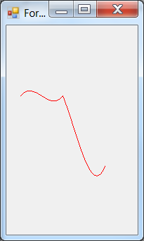
We can lay an interpolation curve to the series of points in a way that the curve passes through the points and in each point the tangent of the curve is proportional to the vector defined by the two neighbouring points, in this case the curve is called cardinal spline. Looking at the parametric description of the curve according to time we can say that at the time t k the curve passes through the point of P k (Figure IV.48, “The cardinal spline”). If the tangent of the curve is V k , at the time t k then the tangent is defined by the equation (IV.4.13).
|
|
(IV.4.13) |

where f(<1) is the tension of the curve. If f=0, then it is just the Catmull-Rom spline [4.4.] .
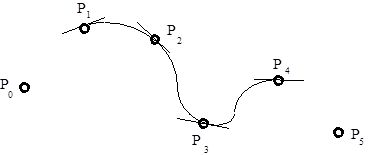
The (IV.4.14) equations contain the parametric description of the cardinal spline:
|
|
(IV.4.14) |


Az usual, at the edges the tangent is calculated by the one-sided difference and this way the curve passes through every point. The advantage of using cardinal splines is that there is no need to solve the system of equations, the curve passes through all the points. Its disadvantage however is that they can be derived continously only once.
The
void AddCurve(array<Point>^ points,
[[int offset, int numberOfSegments],
float tension]);
void AddCurve(array<PointF>^ points,
[[int offset, int numberOfSegments],
loat tension]);
methods add a cardinal spline to the figure. The points array contains the support points, the optional tension parameter contains the tension; and the optional offset parameter defines from which point we would like to consider the points in the points array. We can also set with the numberOfSegments parameter the number of the curve sections we want (that is, how long shall we consider the elements of the points array). By omitting the tension parameter (or setting it to 0), we can define a Catmull-Rom curve.
A closed cardinal spline is added to the figure with the methods:
void AddClosedCurve(array<Point>^ points, float tension);
void AddClosedCurve(array<PointF>^ points, float tension);
The following example lays a (Catmull-Rom) cardinal spline to the points of the previous example (Figure IV.49, “Catmull-Rom spline”).
private: System::Void Form1_Paint(System::Object^ sender,
System::Windows::Forms::PaintEventArgs^ e) {
array<Point>^ pontok = {Point(20,100), Point(40,75),
Point(60,125), Point(80,100),
Point(100,150), Point(120,250),
Point(140,200)};
GraphicsPath^ cPath = gcnew GraphicsPath;
cPath->AddCurve( pontok);
Pen^ cToll = gcnew Pen( Color::Blue );
e->Graphics->DrawPath( cToll, cPath );
}
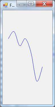
We can add text to the figure with the methods:
void AddString(String^ s, FontFamily^ family, int style,
float emSize, Point origin, StringFormat^ format);
void AddString(String^ s, FontFamily^ family, int style,
float emSize, PointF origin, StringFormat^ format);
void AddString(String^ s, FontFamily^ family, int style,
float emSize, Rectangle layoutRect,
StringFormat^ format);
void AddString(String^ s, FontFamily^ family, int style,
float emSize, RectangleF layoutRect,
StringFormat^ format);
The s parameter is the reference to the string to be printed out. We will talk about the features of letters and fonts later, for now we just share information that are necessary for our current example. The family reference contains the font family of the print out. We can create a similar one using the name of an already existing font family (see the next example). The style parameter is an element of the FontStyle enumeration (FontStyle::Italic, FontStyle::Bold …), the emSize is the vertical size of the rectangle enclosing the letter. We can define the location of the print out either with the Point(F) type origin parameter or with the Rectangle(F) layoutRect parameter. The format parameter is a reference to the instance of the StringFormat class, we can use the StringFormat::GenericDefault property.
The next example fits the GDI+ and Drawing words into a figure and draws it:
private: System::Void Form1_Paint(System::Object^ sender,
System::Windows::Forms::PaintEventArgs^ e) {
GraphicsPath^ sPath = gcnew GraphicsPath;
FontFamily^ family = gcnew FontFamily( "Arial" );
sPath->AddString("GDI+", family, (int)FontStyle::Italic,
20, Point(100,100),
StringFormat::GenericDefault);
sPath->AddString("drawing", family, (int)FontStyle::Italic,
20, Point(160,100),
StringFormat::GenericDefault);
Pen^ cToll = gcnew Pen( Color::Blue );
e->Graphics->DrawPath( cToll, sPath );
}
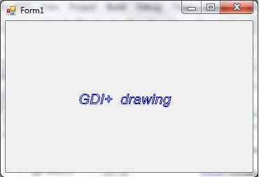
We can add a figure (addingPath) to the current figure instance with the method:
void AddPath(GraphicsPath^ addingPath, bool connect);
The connect parameter caters for making the two elements connected. The following exaple connects two wedges.
private: System::Void Form1_Paint(System::Object^ sender,
System::Windows::Forms::PaintEventArgs^ e) {
array<Point>^ tomb1 = {Point(100,100), Point(200,200),
Point(300,100)};
GraphicsPath^ Path1 = gcnew GraphicsPath;
Path1->AddLines( tomb1 );
array<Point>^ Tomb2 = {Point(400,100), Point(500,200),
Point(600,100)};
GraphicsPath^ Path2 = gcnew GraphicsPath;
Path2->AddLines( Tomb2 );
Path1->AddPath( Path2, true ); // false
Pen^ Toll = gcnew Pen( Color::Green);
e->Graphics->DrawPath( Toll, Path1 );
}
We can widen the figure creating an outline around the original lines (the same applies to the lines of the string characters) possibly at a given distance and after a given geometric transformation. This can be achieved with the method:
void Widen(Pen^ pen[, Matrix^ matrix[, float flatness]]);
The width of the pen parameter gives the distance between the existing lines and the new outline, and the optional matrix parameter defines a transformation before widening. The flatness parameter defines how accurately the outline follows the original curve (this can transform a circle into a polygon). The next example widens two circles while translating (Figure IV.52, “Widened figure”):
private: System::Void Form1_Paint(System::Object^ sender,
System::Windows::Forms::PaintEventArgs^ e) {
GraphicsPath^ Path = gcnew GraphicsPath;
Path->AddEllipse( 0, 0, 100, 100 );
Path->AddEllipse( 100, 0, 100, 100 );
e->Graphics->DrawPath( gcnew Pen(Color::Black), Path );
Pen^ widenPen = gcnew Pen( Color::Black,10.0f );
Matrix^ widenMatrix = gcnew Matrix;
widenMatrix->Translate( 50, 50 );
Path->Widen( widenPen, widenMatrix, 10.0f );
e->Graphics->DrawPath( gcnew Pen( Color::Red ), Path );
}
If we do not want to get a parallel outline but want to replace the figure with a sequence of connected line segments, then we can use the method:
void Flatten([Matrix^ matrix[, float flatness]]);
The interpretation of the parameters is the same as mentioned already when explaining the Widen() method.
We can apply transformations to the current figure with the method:
void Transform(Matrix^ matrix);
We can also distort the figure with the method:
void Warp(array<PointF>^ destPoints, RectangleF srcRect[,
Matrix^ matrix[, WarpMode warpMode[,
float flatness]]]);
In this case the srcRect rectangle is transformed to a quadrangle defined by the destPoints point array as if the plane were made from rubber. Moreover we can apply any geometric transformation using the optional matrix parameter. The warpMode optional parameter can be WarpMode::Perspective (this is the default one) and WarpMode::Bilinear as shown in the equation IV.4.15. We can also define the accuracy of the splitting into segments with the flatness optional parameter.
|
|
(IV.4.15) |

In the next example a text is distorted as defined by the related rectangle (black) and quadrangle (red) in a perspective method and translated.
private: System::Void Form1_Paint(System::Object^ sender,
System::Windows::Forms::PaintEventArgs^ e) {
GraphicsPath^ myPath = gcnew GraphicsPath;
RectangleF srcRect = RectangleF(10,10,100,200);
myPath->AddRectangle( srcRect );
FontFamily^ family = gcnew FontFamily( "Arial" );
myPath->AddString("Distortion", family, (int)FontStyle::Italic,
30,Point(100,100),StringFormat::GenericDefault);
e->Graphics->DrawPath( Pens::Black, myPath );
PointF point1 = PointF(200,200);
PointF point2 = PointF(400,250);
PointF point3 = PointF(220,400);
PointF point4 = PointF(500,350);
array<PointF>^ destPoints = {point1,point2,point3,point4};
Matrix^ translateMatrix = gcnew Matrix;
translateMatrix->Translate( 20, 0 );
myPath->Warp(destPoints, srcRect, translateMatrix,
WarpMode::Perspective, 0.5f );
e->Graphics->DrawPath( gcnew Pen( Color::Red ), myPath );
}
With the help of the GraphicsPathIterator class we can go through the points of the figure, we can set markers with the a SetMarker() method and we can slice the figure with the NextMarker() method. The ClearMarker() method removes the markers.
Within one figure we can define more subfigures that can be opened with the method:
void StartFigure();
We can make the figure closed by connecting the last and the first point by a line using the method:
void CloseFigure();
Each figure that is currently opened will be closed by the method:
void CloseAllFigures();
These last two methods start a new subfigure automatically.
The GetBounds() method gives back the bounding rectangle of the figure:
RectangleF GetBounds([Matrix^ matrix[, Pen^ pen]]);
The optional matrix parameter specifies a transformation to be applied to this path before the bounding rectangle is calculated. The width of the optional pen parameter will raise the size of the bounding rectangle on each side.
The
bool IsVisible(Point point[, Graphics ^ graph]);
bool IsVisible(PointF point[, Graphics ^ graph]);
bool IsVisible(int x, int y[, Graphics ^ graph]);
bool IsVisible(float x, float y[, Graphics ^ graph]);
methods will return true values, if the point of x and y coordinates or defined by the point parameter is contained within this figure. The optional graph parameter defines a drawing paper with a current clipping area, where we test the visibility (the concept of ClipRegion will be described in the next chapter).
The
bool IsOutlineVisible(Point point, Pen^ pen);
bool IsOutlineVisible(PointF point, Pen^ pen);
bool IsOutlineVisible(int x, int y, Pen^ pen);
bool IsOutlineVisible(float x, float y, Pen^ pen);
bool IsOutlineVisible(Point point, Pen^ pen
[, Graphics ^ graph]);
bool IsOutlineVisible(PointF point, Pen^ pen
[, Graphics ^ graph]);
bool IsOutlineVisible(int x, int y, Pen^ pen
[, Graphics ^ graph]);
bool IsOutlineVisible(float x, float y, Pen^ pen
[, Graphics ^ graph]);
methods will return true values if the point of x and y coordinates or defined by the point parameter is contained within (under) the outline of this figure. The optional graph parameter defines a drawing paper with a current clipping area, where we test the visibility
The
void Reverse();
method reverses the order of the points of the figure (in the PathPoints array property).
The
void Reset();
method deletes all the data of the figure.
IV.4.8. Regions
The region class (System::Drawing::Region) models the interior area of a graphics shape composed of rectangles and closed paths (contour), this way the area of the region might be of a complex shape.
We can create instances of the region using the following constructors:
Region();
Region(GraphicsPath^ path);
Region(Rectangle rect);
Region(RectangleF rect);
Region(RegionData^ rgnData);
If we do not define any parameter, then an empty region will be created. The path and the rect parameters define the initial shape of the region.
We can set the clipping region with the methods of the Graphics class:
void SetClip(Graphics^ g[, CombineMode combineMode]);
void SetClip(GraphicsPath^ path[, CombineMode combineMode]);
void SetClip(Rectangle rect[, CombineMode combineMode]);
void SetClip(RectangleF rect[, CombineMode combineMode]);
void SetClip(Region^ region, CombineMode combineMode);
This way our shape can be used as a special picture-frame. The geometry of the picture-frame is defined by the picture-frame of another drawing paper (parameter g), the figure (path), the rectangle (rect) or the region (region). The combineMode parameter (optional for all methods except for the last) may have the values of the of the CombineMode enumeration:
The
Replace(the currecnt clipping region (picture-frame) is replaced by the given geometry parameter G),Intersect(the current picture-frame – R – intersects with the given geometry – G: ),
),Union(union with the given geometry ),
Xor(symmetric difference with the given geometry ),
),Exclude(the difference between the existing and the given region ) and
) andComplement(the difference between the given and the existing region ).
).
Windows can use a region to refresh the drawing.
The RegionData class contains a byte array in the Data property and this array describes the data of the region.
The
RegionData^ GetRegionData()
method returns an instance of the RegionData class, which describes to the current region. The
array<RectangleF>^ GetRegionScans(Matrix^ matrix)
method approximates the selected region with the array of rectangles. The matrix parameter contains the matrix of a previous transformation.
The
void MakeEmpty()
method turns the current region into an empty one, whereas the
void MakeInfinite()
method turns the current region to an infinite one.
We can perform operations with the regions. As the result of the query of the following methods
void Complement(Region^ region);
void Complement(RectangleF rect);
void Complement(Rectangle rect);
void Complement(GraphicsPath^ path);
the current region will be the intersection of the geometry defined as parameter and the complementer of the current region. That is, the current region will be the difference of the geometry and the current region. (Let’s have R as the set of the points of the current region, and G to be the set of the given geometry, then we can describe this operation as  ).
).
With the
void Exclude(Region^ region);
void Exclude(RectangleF rect);
void Exclude(Rectangle rect);
void Exclude(GraphicsPath^ path);
methods the current region will be the intersection of the current region and the complementer of the shape defined as parameter, that is, the result will be the difference of the current region and the given geometry ( ).
).
With the
void Intersect(Region^ region);
void Intersect(RectangleF rect);
void Intersect(Rectangle rect);
void Intersect(GraphicsPath^ path);
methods the current region will be the intersection of itself and the geometry defined as parameter ( ).
).
With the
void Union(Region^ region);
void Union(RectangleF rect);
void Union(Rectangle rect);
void Union(GraphicsPath^ path);
methods the current region will be the union of itself and the geometry defined as parameter ( ).
).
With the
void Xor(Region^ region);
void Xor(RectangleF rect);
void Xor(Rectangle rect);
void Xor(GraphicsPath^ path);
methods the current region will contain only those points that were only in one of the geometries. That geometry can be achieved by removing the intersection of the current region and the given geometry from the union of the current region and the given geometry (symmetric difference  ).
).
We can transform the region with a transformation matrix or with given translation coordinates:
void Transform(Matrix^ matrix);
void Translate(int dx, int dy);
void Translate(float dx, float dy);
We can examine if a point is included in the current region with the methods:
bool IsVisible(Point point[, Graphics gr]);
bool IsVisible(PointF point[, Graphics gr]);
bool IsVisible(float x, float y);
bool IsVisible(int x, int y[, Graphics gr]);
We can decide if rectangles intersect with the current region using the methods:
bool IsVisible(Rectangle rect[, Graphics gr]);
bool IsVisible(RectangleF rect[, Graphics gr]);
bool IsVisible(int x, int y, int width, int height
[, Graphics gr]);
bool IsVisible(float x, float y, float width, float height
[, Graphics gr]);
In both cases the we can define the drawing paper with the optional Graphics type parameter.
The
bool IsEmpty(Graphics^ g);
method tests if the current region is empty or not, whereas the
bool IsInfinite(Graphics^ g);
method tests if it is infinite or not.
The following example creates a figure using text and defines a clipping region before to draw the figure:
private: System::Void Form1_Paint(System::Object^ sender,
System::Windows::Forms::PaintEventArgs^ e) {
GraphicsPath^ sPath = gcnew GraphicsPath;
FontFamily^ family = gcnew FontFamily( "Arial" );
sPath->AddString("Clipped text", family, (int)FontStyle::Italic,
40,Point(0,0),StringFormat::GenericDefault);
System::Drawing::Region ^ clip = gcnew System::Drawing::Region(
Rectangle(20,20,340,15));
e->Graphics->SetClip(clip, CombineMode::Replace);
e->Graphics->DrawPath( gcnew Pen(Color::Red), sPath );
}
IV.4.9. Image handling (Image, Bitmap, MetaFile, Icon)
There are two basic strategies to store images. In the first case the image is stored in a way like it was drawn with a pencil. In this case the storage of the image data happens in a way that the data of the line segments needed to draw the image (vectors) are stored and based on these we can draw the picture. This method of storage is called vector image storage. Figure IV.55, “Vectorial A” shows the vectorial drawing of capital A.

We also have the possibility to divide the image into pixels (raster points) and to store the color of each and every pixel. This rasterized picture is called bitmap considering its similarity to maps. Figure IV.56, “Rasterized A” shows the black and white bitmap of the capital A.
The Image is an abstract image storing class. It is the parent of the rasterized System::Drawing::Bitmap and vectorial System::Drawing::Imaging::MetaFile classes that contain Windows drawings. In order to create Image objects we can use the static methods of the Image class and with these we can load images from the given files (filename).
static Image^ FromFile(String^ filename
[, bool useEmbeddedColorManagement]);
static Image^ FromStream(Stream^ stream
[, bool useEmbeddedColorManagement
[, bool validateImageData]]);
If the useEmbeddedColorManagement logical variable is true then the color handling information of the file is used by the method, otherwise not (the true value is the default one). In case of stream the validateImageData logical variable controls the data check of the image. Data check works by default. We can also use the old GDI bitmaps with the FromHbitmap() method.
We can draw the loaded bitmaps with the Graphics::DrawImage(Image,Point) method. The next example loads the image of the Visual Studio development environment to the form (Figure IV.57, “Image on the form”).
private: System::Void Form1_Paint(System::Object^ sender,
System::Windows::Forms::PaintEventArgs^ e) {
Image^ kep = Image::FromFile( "C:\\VC++.png" );
e->Graphics->DrawImage( kep, Point(10,10) );
}
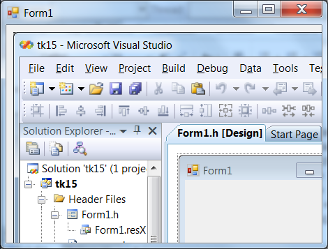
Properties of the Image class store the data of the image. The int type Width and Height read only properties define the width and the height of the image in pixels. The Size structure type Size ready only property also stores the size data. The float type HorizontalResolution and VerticalResolution properties define the resolution of the image in pixel/inch dimension. The SizeF structure type PhisicalDimension read only property defines the real size of the image, in case of bitmap it is defined in pixels whereas in case of metafile picture it is defined in 0.01 mm units.
With the ImageFormat class type RawFormat property we can specify the file format of the image, which can be used when storing the image. The Bmp property of the
ImageFormat
class specifies a bitmap, the Emf specifies an extended metafile, the Exif specifies an exchangeable image file. We can use the Gif property for the standard image format (Graphics Interchange Format). The Guid property contains the global object identifier applied by Microsoft. We can use the Icon property for the Windows icons. The Jpeg property specifies the format of the JPEG (Joint Photographic Experts Group) standard, the MemoryBmp property specifies the format of the memory bitmaps and the Png property belongs to PNG format of W3C (World Wide Web Consortium
[4.5.]
) for transmission of graphical elements through the network (Portable Network Graphics). The Tiff property specifies the format of the TIFF (Tagged Image File Format) standard, whereas the Wmf property specifies the format of the Windows metafiles.
The bits of the int type Flags property specifies the attributes of the pixel data stored in the image (color handling, transparency, enlargement etc.). Some constants adequate for a typical bit state are the ImageFlagsNone (0), the ImageFlagsScalable (1), the ImageFlagsHasAlpha (2) and the ImageFlagsColorSpaceRGB (16).
Images can store their colors in the color palette related to the image. The ColorPaletteClass type Palette property is nothing but a color array (array<Color>^ Entries) that contain the colors. The ColorPaletteClass also has a Flags property. The interpretation of this by bits is as follows: the color contains alpha information (1), the color defines a grayscale (2), the color gives the so called halftone
[4.6.]
information when the colors percieved by human eyes as grayscale are built from black and white elements (Figure IV.58, “Halftone representation”).
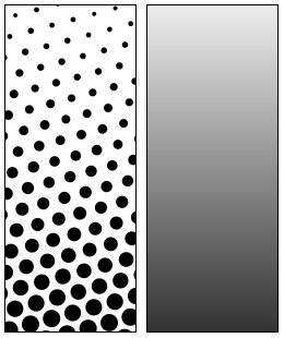
The bounds of the picture defined in the given graphical units returns the method:
RectangleF GetBounds(GraphicsUnit pageUnit);
The
static int GetPixelFormatSize(PixelFormat pixfmt);
method defines how the image is stored, this can be a palette index or the value of the color itself. Some possible values: Gdi – the pixel contains GDI color code (rgb), Alpha – the pixel contains trasnparency information too, Format8bppIndexed – index, 8 bits per pixel color(256 colors).
With the following methods we can query if the image is transparent
static bool IsAlphaPixelFormat(PixelFormat pixfmt);
if the pixel format of the image is 32 bits
static bool IsCanonicalPixelFormat(PixelFormat pixfmt);
if the pixel format of the image is 64 bits
static bool IsExtendedPixelFormat(PixelFormat pixfmt);
With the
void RotateFlip(RotateFlipType rotateFlipType);
method we can rotate and flip the image according to the elements of the RotateFlipType enumeration (e.g Rotate90FlipNone rotates with 90 degrees and does not do flipping, RotateNoneFlipX flips to the y axis, Rotate90FlipXY rotates with 90 degrees and flips centrally).
The next example displays the image of Figure IV.57, “Image on the form” form flipping it to the y axis:
private: System::Void Form1_Paint(System::Object^ sender,
System::Windows::Forms::PaintEventArgs^ e) {
Image^ kep = Image::FromFile( "C:\\VC++.png" );
kep->RotateFlip(RotateFlipType::RotateNoneFlipX);
e->Graphics->DrawImage( kep, Point(10,10) );
}
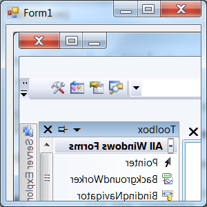
We can save the images into files with the
void Save(String^ filename[,ImageFormat^ format]);
method. The filename parameter contains the name of the file, the file extension depends on the extension in the filename. We can define the saving format with the optional format parameter. If there is no coding information defined for the file formats (like e.g. Wmf) then the method saves into Png format.
We can also save the data of the image into a stream with the method:
void Save(Stream^ stream, ImageFormat^ format);
While the Bitmap is the descendant of the Image class, it inherits all the properties and functions of the Image, however the data structure of the Bitmap corresponds to method of storing data in the memory, which gives the possibility to use a set of special methods as well. The Bitmap class have constructors and with their help we can create a bitmap from Image, from Stream, from a file, moreover from any graphics or from pixel data stored in the memory.
The following constructor creates an empty bitmap with given size (width, height parameters):
Bitmap(int width, int height[,, PixelFormat format]);
if we use the PixelFormat type format parameter, then we can specify the color depth as we could see it at the Image::GepPixelFormat() method.
The
Bitmap(Image^ original);
Bitmap(Image^ original, Size newSize);
Bitmap(Image^ original, int width, int height);
constructors create a bitmap from the Image defined as parameter. If we define the newSize parameter or the width and height parameters, then the bitmap is created with the rescaling of the image to the new size.
With the
Bitmap(Stream^ stream[, bool useIcm]);
overloaded constructor we can create a bitmap from a stream, and with the
Bitmap(String^ filename[, bool useIcm]);
overloaded constructor we can create it from a file. If we use the useIcm logical parameter, then we can specify whether to use color correction or not.
We can create a bitmap of any Graphics instance, for example of the screen with the
Bitmap(int width, int height, Graphics^ g);
constructor. The integers of width and height define the size, the g parameter define the instance of the drawing paper, the DpiX and DpiY properties of this define the bitmap resolution. We can also create a bitmap from the memory referenced by the scan0 pointer that points to the integer, if we set the width, the height and the stride (difference between two bitmap rows) in bytes:
Bitmap(int width, int height, int stride,
PixelFormat format, IntPtr scan0);
The resolution of a newly created bitmap can be set with the method:
void SetResolution(float xDpi, float yDpi);
The xDpi and yDpi parameters are in dot per inch units.
Some methods not inhereted from the Image class can supplement the opportunities offered by bitmaps. We can reach one point of the bitmap directly. The color of the given pixel (x, y) is returned by the method:
Color GetPixel(int x, int y);
We can set the color of the specified pixel with the method:
void SetPixel(int x, int y, Color color);
The
void MakeTransparent([Color transparentColor]);
function makes the default transparent color transparent for this Bitmap. If we also define the transparentColor parameter, then this color will be transparent.
The next example loads a bitmap and draws it. After it the points of the bitmap colored to a color that is close to white will be painted green and then the program draws the modified bitmap. In the next step it makes the green color transparent and draws the bitmap again moved with half of the size (Figure IV.60, “Coloring bitmap”).
private: System::Void Form1_Click(System::Object^ sender,
System::EventArgs^ e) {
Bitmap ^ bm = gcnew Bitmap("C:\\D\\X.png");
Graphics ^ g = this->CreateGraphics();
g->DrawImage( bm, Point(0,0) );
Color c;
for (int i=0; i<bm->Width; i++) {
for (int j=0; j<bm->Height; j++) {
Color c=bm->GetPixel(i,j);
if ((c.R>200)&&(c.G>200)&&(c.B>200))
bm->SetPixel(i,j,Color::Green); }
}
g->DrawImage( bm, Point(bm->Width,bm->Height) );
}
Bitmap handling with the GetPixel() and SetPixel() methods is not effective enough. We have the option to load the bits of the bitmap into the memory and to modify them, then we can pump the bits back to the bitmap. In this case we need to ensure that the operating system does not disturb our actions. In order to store the bitmaps in the memory we can use the function:
BitmapData^ LockBits(Rectangle rect, ImageLockMode flags,
PixelFormat format[, BitmapData^ bitmapData]);
void UnlockBits(BitmapData^ bitmapdata);
Where the rect parameter selects the part of the bitmap we would like to store, the enumeration type ImageLockMode flags parameter defines the way of data handling (ReadOnly, WriteOnly, ReadWrite, UserInputBuffer). We are already familiar with the PixelFormat enumeration. The BitmapData class type bitmapdata optional parameter has the properties: Height and Width are the size of the bitmap, the Stride is the width of the scanline, whereas scan0 is the address of the first pixel. The returned value contains the data of the bitmap in an isntance of the BitmapData reference class.
After calling the function the bitmapdata is locked and it can be manipulated with the methods of the
System::Runtime::InteropServices
::Marshal class. With the methods of the Marshal class we can allocate a non-managed memory block, we can copy the non-managed memory blocks, or we can copy managed memory objects to a non-managed memory area. For example the
static void Copy(IntPtr source,
array<unsigned char>^ destination,
int startIndex, int length);
method of the Marshal class copies length bytes from the startIndex position of the memory area pointed by the source pointer to the destination managed array, whereas the
static void Copy(array<unsigned char>^ source,
int startIndex,
IntPtr destination, int length);
method copies length bytes in reverse order from the source managed array from the startindex position to the destination non-managed area.
Once we copied the parts from the bitmap that we intended to modify, we modified them and copied them back, then we can unlock the locked memory with the method:
void UnlockBits(BitmapData^ bitmapdata);
The following example draws a managed bitmap that was loaded to the memory when clicking on the form. After it locks it, copies the bytes of the image, erases the middle third of the image, stores the data back into the bitmap, unlocks the memory and draws the bitmap.
private: System::Void Form1_Click(System::Object^ sender,
System::EventArgs^ e) {
Bitmap ^ bm = gcnew Bitmap("C:\\D\\X.png");
Graphics ^ g = this->CreateGraphics();
g->DrawImage( bm, Point(0,0) );
Rectangle rect = Rectangle(0,0,bm->Width,bm->Height);
System::Drawing::Imaging::BitmapData^ bmpData = bm->LockBits(
rect, System::Drawing::Imaging::ImageLockMode::ReadWrite,
bm->PixelFormat );
IntPtr ptr = bmpData->Scan0;
int bytes = Math::Abs(bmpData->Stride) * bm->Height;
array<Byte>^Values = gcnew array<Byte>(bytes);
System::Runtime::InteropServices::Marshal::Copy( ptr, Values, 0, bytes );
for ( int counter = Values->Length/3; counter < 2*Values->Length/3; counter ++ )
{
Values[ counter ] = 255;
}
System::Runtime::InteropServices::Marshal::Copy( Values, 0,
ptr, bytes );
bm->UnlockBits( bmpData );
g->DrawImage( bm, bm->Width, 0 );}
We can also work with metafiles because we can use the methods of the Image class. The next example loads a Png file into a bitmap and saves it as a Wmf metafile.
private: System::Void Form1_Click(System::Object^ sender,
System::EventArgs^ e) {
Bitmap ^ bm = gcnew Bitmap("C:\\D\\X.png");
Graphics ^ g = this->CreateGraphics();
g->DrawImage( bm, bm->Width, 0 );
bm->Save("C:\\D\\X.wmf");
}
IV.4.10. Brushes
Brushes can be used to paint areas in GDI+
[4.1.]
. Each brush type is a descendant of the System::Drawing::Brush class (Figure IV.27, “The classes of GDI+”). The simplest brush is of a single color (SolidBrush). The constructor of this creates a brush from the given color. Accordingly the Color property of the class picks up the color of the brush.
SolidBrush(Color color);
The following example paints a red rectangle on the form with the FillRectangle() method of the Graphics class (Figure IV.62, “Brushes”).
private: System::Void Form1_Paint(System::Object^ sender,
System::Windows::Forms::PaintEventArgs^ e) {
SolidBrush ^ sb = gcnew SolidBrush(Color::Red);
e->Graphics->FillRectangle(sb,200,20,150,50);
}
HatchBrush, the patterned brush is also a descendant of the Brush class and it is defined in the System::Drawing::Drawing2D namespace, that is why it is necessary to specify:
using namespace System::Drawing::Drawing2D;
The constructor of the patterned brush defines the pattern of the brush, the color of the pattern and the background. If we omit the last parameter (squared brackets mark the optional parameters), then the background color will be black:
HatchBrush(HatchStyle hatchstyle, Color foreColor,
[Color backColor])
The HatchStyle enumeration of the Drawing2D namespace contains a lot of predefined patterns. The horizontal one is the HatchStyle::Horizontal, the vertical one is Vertical, the diagonal one (leaning to the left) is the ForwardDiagonal etc. The next example paints a yellow rectangle with a red diagonal-hatched brush (Figure IV.62, “Brushes”).
private: System::Void Form1_Paint(System::Object^ sender,
System::Windows::Forms::PaintEventArgs^ e) {
HatchBrush ^ hb = gcnew HatchBrush(HatchStyle::ForwardDiagonal,
Color::Red,Color::Yellow);
e->Graphics->FillRectangle(hb,200,80,150,50);
}
The characteristic properties of the patterned brushes are the BackGroundColor for the color of the background, the ForegroundColor for the color of the foreground and HatchStyle for the pattern type.
We can create brushes painting with images using the instances of the TextureBrush class. These are its constructors:
TextureBrush(Image^ image);
TextureBrush(Image^ image, WrapMode wrapMode);
TextureBrush(Image^ image, Rectangle dstRect);
TextureBrush(Image^ image, RectangleF dstRect);
TextureBrush(Image^ image, WrapMode wrapMode,
Rectangle dstRect);
TextureBrush(Image^ image, WrapMode wrapMode,
RectangleF dstRect);
TextureBrush(Image^ image, Rectangle dstRect,
ImageAttributes^ imageAttr);
TextureBrush(Image^ image, RectangleF dstRect,
ImageAttributes^ imageAttr);
The image defines the picture used for painting, the dstRect defines the distortion of the picture when painting. The wrapMode parameter specifies how the images used for painting are tiled. (The members of the WrapMode enumeration: Tile – as if it was built from tiles, TileFlipX – built from tiles mirrored to the y axis, TileFlipY - built from tiles mirrored to the x axis, TileFlipXY – built from centrally mirrored tiles, Clamped – the texture is not built from tiles). The
System::Drawing::Imaging
::ImageAttributes^ type imageAttr contains additional information about the image (colors, color corrections, painting methods etc).
The Image (Image^ type) property of the TextureBrush class defines the graphics of the painting, the Transform^ type Transform property and its methods can be used similarly to their usage already discussed for transformations. The WrapMode property contains the arrangement.
The following example paints a rectangle with images (Figure IV.62, “Brushes”).
private: System::Void Form1_Paint(System::Object^ sender,
System::Windows::Forms::PaintEventArgs^ e) {
Image ^ im = Image::FromFile("c:\\M\\mogi.png");
TextureBrush ^ tb = gcnew TextureBrush(im);
Matrix ^ m= gcnew Matrix();
m->Translate(5,5);
tb->Transform->Reset();
tb->Transform=m;
Graphics ^ g = this->CreateGraphics();
g->FillRectangle(tb, 200, 140, 150, 50);
}
The Drawing2D namespace contains the LinearGradientBrush class. With its constructors we can create gradient brushes. With the various constructors we can set different gradient types. The System::Windows::Media::BrushMappingMode enumeration defines a coordinate systems for the gradient effect. The elements of this enumertion are Absolute and RelativeToBoudingBox. The Absolute means the points are interpreted in the current coordinate system. When the RelativeToBoudingBox is set, the top left corner of the bounding rectangle of the given painting will be (0,0), whereas the bottom right corner will be (1,1).
The linear gradient brushes can be created with different constructor calls. Using the constructors
LinearGradientBrush(Rectangle rect,
Color startColor, Color endColor,
double angle, [isAgleScaleable]);
LinearGradientBrush(RectangleF rect,
Color startColor, Color endColor,
double angle, [isAgleScaleable]);
we can set the starting color (startColor) and the ending color (endColor). In the RelativeToBoudingBox brush coordinate system the angle of the gradient is given in degrees (0 is a horizontal gradient, 90 is vertical).
Using the following constructors
LinearGradientBrush(Point startPoint, Point endPoint,
Color startColor, Color endColor);
LinearGradientBrush(PointF startPoint, PointF endPoint,
Color startColor, Color endColor);
LinearGradientBrush(Rectangle rect,
Color startColor, Color endColor
LinearGradientMode lgm);
LinearGradientBrush(RectangleF rect,
Color startColor, Color endColor,
LinearGradientMode lgm);
we can set the starting color (startColor) and the ending color (endColor) too. In the RelativeToBoudingBox brush coordinate system we can set the angle of the gradient with the points startPoint and endPoint or with the corners of rect in the units of %. The elements of the LinearGradientMode enumeration (Horizontal, Vertical, ForwardDiagonal, BackwardDiagonal) define the direction of the color transition.
With the
PathGradientBrush(GraphicsPath path);
PathGradientBrush(Point[] points);
PathGradientBrush(PointF[] points);
PathGradientBrush(Point[] points, WrapMode wrapMode);
constructors we can create a brush which changes its color along a curve. We can define the curve with the path and the points parameters. We already got familiar with the wrapMode WrapMode type parameter when discussing the texture brushes.
Both gradient brushes have a WrapMode property that defines the method how to repeat the painting and they also have a Transform feature that contains local transformation. Both gradient brushes contain Blend^ type Blend property. The Factors and Positions properties of the Blend class are float arrays with elements between 0 and 1, which define the intensity of the color in % and the length position in %. Both gradient brushes have an InterpolationColors (ColorBlend class type) property where we can set the colors besides the positions in % instead of the color intensity. Both gradient brushes have a bounding Rectangle property.
The Color array type SurroundColors property of the PathGradientBrush contains the applied colors.
A brush can be transparent, if we use ARGB colors. The following example draws a transparent rectangle on the top of the rectangles painted differently.
private: System::Void Form1_Paint(System::Object^ sender,
System::Windows::Forms::PaintEventArgs^ e) {
SolidBrush ^ sb = gcnew SolidBrush(Color::Red);
e->Graphics->FillRectangle(sb,200,20,150,50);
HatchBrush ^ hb = gcnew HatchBrush(
HatchStyle::ForwardDiagonal,
Color::Red,Color::Yellow);
e->Graphics->FillRectangle(hb,200,80,150,50);
Image ^ im = Image::FromFile("c:\\M\\mogi.png");
TextureBrush ^ tb = gcnew TextureBrush(im);
Matrix ^ m= gcnew Matrix();
m->Translate(5,5);
tb->Transform->Reset();
tb->Transform=m;
e->Graphics->FillRectangle(tb, 200, 140, 150, 50);
LinearGradientBrush ^ lgb = gcnew LinearGradientBrush(
PointF(0,0), PointF(100,100), Color::Blue, Color::Red);
e->Graphics->FillRectangle(lgb, 200, 200, 150, 50);
SolidBrush ^ at = gcnew SolidBrush(
Color::FromArgb(127,Color::Red));
e->Graphics->FillRectangle(at, 250, 10, 200, 270);
}
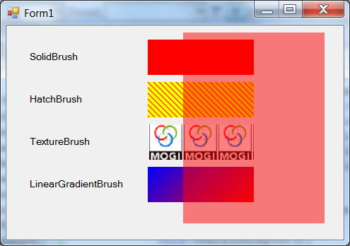
IV.4.11. Pens
We can draw line pictures with pens. The pens have color and width. With the
Pen(Brush brush [, float width]);
Pen(Color color [, float width]);
constructors of the Pen class we can create a pen defined by its color or its brush. We can also specify the width of the pen. The Brush, Color and Width properties store the mentioned features of the pen.
The DashStyle property can set with one of the elements of the DashStyle enumeration (
System::Drawing::Drawing2D
namespace). We can set this way the pattern of the pen (Solid – continuous, Dash – dashed, Dot – dotted, DashDot – dashes and dots, DashDotDot – dashes and double dots, and Custom). In case of the the last dash style we can define the pattern, with the consecutive elements of the DashPattern float array consisting the length of dashes and spaces.
With the float type DashOffset property we can set the distance between the starting point of the line and starting point of the dash. In case of dashed lines we can also set the cap style used at the end of the dashes with the DashCap (
System::Drawing::Drawing2D
). The elements of the DashCap enumeration are: Flat – flat, Round - rounded, Triangle – triangular.
The Alignment property can be a value of the PenAligment type enumeration (
System::Drawing::Drawing2D
namespace), and it specify where to put the line concerning the edge of the shape (Center – centered over the line, Inset – in the inside of a closed shape, OutSet – outside of a closed shape, Left – to the left of the line, Right – to the right of the line).
In order to achieve a joint geometry of the consecutive lines of the shapes we can use the LineJoin property of the LineJoin enumeration type (Bevel – a corner clipped in a certain angle, Round – rounded, Miter and MiterClipped also mean a clipped connection, if the length of the miter exceeds the float type MiterLimit value).
In order to control the drawing of the line endings the StartCap and the EndCap
System::Drawing::Drawing2D::LineCap
enumeration type properties can be used (Flat – flat, Square - square, Round – rounded, ArrowAnchor – ending with an arrow, RoundAnchor – ending with a circle etc). The CustomStartCap and the CustomEndCap properties can be interesting and those are instances of the CustomLineCap class. The instance can be created with the
CustomLineCap(GraphicsPath fillPath, GraphicsPath strokePath
[, LineCap baseCap[, float baseInset]]);
constructor. We can define the filling with a figure (fillPath) and the outline (strokePath). We can use an existing line cap (baseCap), or we can insert a gap into the cap and the line (baseInset). The BaseCap property of the CustomLineCap class identifies the parent line cap and the BaseInset contains the gap. We can determine the mode how lines are joined to each other (StrokeJoin), or we can set a scale for their width (WidthScale property). By default this is the width of the line.
The ready only PenType enumeration type PenType property of the Pen class tells us the type of the pen (SolidColor, HatchFill, TextureFill, LinearGradient, PathGradient)
Of course, pens also have a Transform property that defines the local transformation.
The following example draws a line with a red solid pen, then with a pen defined with a linear gradient brush. After this it draws a line on one of the end with an arrow, then on the other end with a rounded cap. Then two dashed lines come, the first with a predefined pattern, whereas the second one with an pattern array. This is followed by two rectangle shapes, one of them with a clipped and default OutSet Alignment property, then the other with the InSet property without clipping (Figure IV.63, “Pens”).
private: System::Void Form1_Paint(System::Object^ sender,
System::Windows::Forms::PaintEventArgs^ e) {
Pen ^ ps = gcnew Pen(Color::Red,5);
e->Graphics->DrawLine(ps,10,25,100,25);
LinearGradientBrush ^ gb = gcnew LinearGradientBrush(
PointF(10, 10), PointF(110, 10),
Color::Red, Color::Blue);
Pen ^ pg = gcnew Pen(gb,5);
e->Graphics->DrawLine(pg,10,50,100,50);
ps->StartCap=LineCap::ArrowAnchor;
pg->EndCap=LineCap::Round;
e->Graphics->DrawLine(pg,10,75,100,75);
pg->DashStyle=DashStyle::DashDot;
e->Graphics->DrawLine(pg,10,100,100,100);
array <float> ^ dp= {1.0f,0.1f,2.0f,0.2f,3.0f,0.3f};
pg->DashPattern=dp;
e->Graphics->DrawLine(pg, 10, 125, 100, 125);
GraphicsPath^ mp = gcnew GraphicsPath;
RectangleF srcRect = RectangleF(10,150,100,20);
mp->AddRectangle( srcRect );
ps->LineJoin=LineJoin::Bevel;
e->Graphics->DrawPath( ps , mp );
Matrix ^ em = gcnew Matrix();
em->Reset();
em->Translate(0,25);
mp->Transform(em);
pg->Alignment=PenAlignment::Inset;
e->Graphics->DrawPath( pg , mp );
}
IV.4.12. Font, FontFamily
We can differentiate three basic types of character sets in Windows. In the first case the information that is necessary to display a character is stored in a bitmap. In the second case the vector based fonts define which lines should be taken to draw the character. In the third case the so called TrueType character set is used which means that the definition of characters consists of the set of points and special algorithms and those are able to define the characters for any type of resolutions.
When using the TrueType character set, then the so called TrueType rasterizer creates a bitmap character set from the points and algorithms according to the requirements. The result of this is that if we plan the page to be printed with a publishing software, then the printout will be the same what was visible on the screen (WYSIWYG - What You See Is What You Get). Microsoft bought the right of using the TrueType fonts from Apple Computer [4.7.] . It is obvious that the first two character representation methods have their advantages and disadvantages as well. It is possible to resize the vector based fonts as wished, however, in a lot of cases their visualization is not aesthetic enough and is not readable. On the other hand, bitmap fonts are well readable but they cannot be deform freely. The usage of the TrueType type character set guarantees the above benefits and eliminates disadvantages.
Let us get familiar with some notions that help us to navigate in the world of fonts. It is a basic question whether the width of the line of the letter can be changed when displaying the character. Is it possible to use a thinner or a thicker letter drawing? The line of the letter is called „stroke” in the English terminology.
There are more character sets that uses small crossing lines to close the line of the letters when drawing them. The letters will have small soles and hat. These small crossing lines are called serif. This way that character set that do not use these closing serifsis called sanserif, that is, without serif.
The rectangular area that bounds the character is called character cell. The size of this can be characterized by the emSize parameter, which shows the size of the character in points (1/72 inch). The em prefix comes from pronounciation of the M letter because it is used to sizing the font. Characters do not fully fill in their cells. The cell is characterized by its width, height and its starting point which is usually the top left corner. The character cell is devided into two parts by a horizontal line. Characters are sitting on this line, that is, the base line. The part above the base line is called ascent and the part below the base line is called descent. The distance of two base lines that are in two character cells placed below each other is called leading. Capital letters written on he base line do not reach the top of the character cell either.
The internal leading is the area between the top edge of the character cell and the top edge of capital letters. If the top and bottom edge of the character cells placed below each other do not touch, then the distance between these two is called the externalleading.
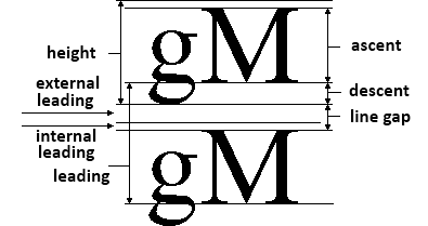
A given size of a character type is called typeface. Windows is capable of creating typefaces with distortion in the given size. Italic letters (italic) are created in a way that the points of the character remain unchanged on the base line, whereas the other parts of the character are slipped depending on their distance from the base line (the character leans). The bold letters (bold) can be easily derived from making the stroke thicker. Obviously it is easy to create underlined and lined strikeout characters with adding a horizontal line to a specific place. The notion of pitch is also in use which is specifying how many characters have to be written next to each other from a given font so that the width of the written text is one inch (~2.54 cm). It is worth mentioning that the logical inch is used for displaying characters on the screen. The size of the logical inch is defined in a way that the text is as well readable on screen as on paper. Two basic font type exist. One is non-proportional – fix sized – in which each character is placed in a cell with the same size, being either an „i” or an „m”. Recently these font types are called monospace fonts. The other is proportional in which case the width of the cell depends on the given letter. In this latest case the average character widths and the average and maximum pitch sizes can be used.
It is worth dealing with the with the aspect ratio of the characters, given that not all the fonts could be displayed on all output devices (e.g dot matrix printer). Windows can perform aspect ratio conversion in order to display successfully. The uses font families depending on the appearance of the characters.
Traditional character sets use the data shown on Figure IV.65, “Traditional character widths” to descript the dimensions of the characters. Instead of this traditional interpretation the TrueType character sets use the so called ABC data. As it is visible on Figure IV.66, “ABC character widths” the A and C values can be negative as well.
Font families contain fonts that have similar characteristics. The .Net defines the FontFamily class to model font families (this class cannot be inherited). We can create FontFamily instances with the
FontFamily(GenericFontFamilies genericFamily);
FontFamily(String^ name[, FontCollection^ fontCollection]);
constructors. We can choose the value of the genericFamily parameter from the elements of the GenericFontFamilies enumeration in order to create a family. The possible values of the enumeration (Serif, SansSerif and Monospace) cover already known notions. The name parameter contain the name of the new font family. It can be an empty string or the name of a font family that has not been installed on the computer or a name of a non TrueType font. We can also create collections from font families. We can define the collection with the fontCollection parameterwhere we can place the new font family.
We can get information opportunities from the properties of the FontFamily class. With the static Families property we can query the font families of the current drawing paper into a FontFamily type array. The FontFamily type, static GenericMonospace, GenericSansSerif and GenericSerif properties give a non proportional, a sansserif and a serif font family. The string type Name property contains the name of the font family.
The static
FontFamily[] GetFamilies(Graphics graphics);
method returns all family font names that can be found on the given drawing paper.
The following example collects the names of all font families of the drawing paper to the listbox when clicking on the form.
private: System::Void Form1_Click(System::Object^ sender,
System::EventArgs^ e) {
Graphics ^ g = this->CreateGraphics();
array <FontFamily ^> ^ f = gcnew array<FontFamily^>(100);
f=FontFamily::GetFamilies(g);
for (int i=0; i<f->GetLength(0); i++) {
listBox1->Items->Add(f[i]->Name);
}
}
The
int GetCellAscent(FontStyle style);
int GetCellDescent(FontStyle style);
int GetEmHeight(FontStyle style);
int GetLineSpacing(FontStyle style);
String^ GetName(int language);
method queries the data defined by the style parameter of the given font family.
The
bool IsStyleAvailable(FontStyle style);
method indicates if the given font family has the given style. The values of the FontStyle enumeration are: Bold, Italic, Underline and Strikeout.
The GDI+ uses the Font class to model the font types. We can create the instances of the class with the constructors:
Font(FontFamily^ family, float emSize[, FontStyle style
[, GraphicsUnit unit [, unsigned char gdiCharSet
[, bool gdiVerticalFont]]]]);
Font(FontFamily^ family, float emSize, GraphicsUnit unit);
Font(String^ familyName, float emSize[, FontStyle style
[, GraphicsUnit unit[, unsigned char gdiCharSet
[, bool gdiVerticalFont]]]]);
Font(String^ familyName, float emSize, GraphicsUnit unit);
Font(Font^ prototype, FontStyle newStyle);
The family parameter defines the familiy of the new font, the familyName defines the name of this family. The emSize is the size of the font in points, the style is the font type (italic, bold etc.). The unit parameter defines the units (Pixel, Inch, Millimeter etc.) used by the font
The gdiCharset indentifies the character set provided by GDI+. The gdiVerticalFont regulates vertical writing. We can define a new font from an existing font and with the new newStyle style.
All properties of the Font class are read-only. If we would like to make changes, then we need to create a new font. The FontFamily^ type FontFamily property identifies the font family. The Name string defines the name of the font, whereas the OriginalFontName string defines the original name of the font. If the IsSystemFont logical property is true then we work with a system font. In this case the SystemFontName string property defines the name of the system font. The GdiVerticalFont logical property defines whether the font is vertical. The GdiCharSet byte type property identifies the GDI character set. The Size (emSize) and the SizeInPonts define the font size in points. The Style logical property indentifies the font style with the elements of the FontStyle type enumeration (Italic, Bold, Underline and Strikeout). The Unit property defines the unit of measure for this font.
The
float GetHeight();
method returns the distance that can be measured between lines in pixels. The
float GetHeight(Graphics^ graphics);
method returns the distance that can be measured between lines in GraphicsUnit type units. The
float GetHeight(float dpi);
method defines the distance that can be measured between lines in pixels on a device with a given dpi (dot per inch – pont per inch) resolution.
The next example shows the distortion of a font chosen by clicking on the Type button with the Bold, Italic and Underline checkboxes. (Figure IV.68, “Font distortions”).
IV.4.13. Drawing routines
The Graphics class offers a set of drawing routines. We can erase the whole drawing paper with a given color (color)
void Clear(Color color);
In the next drawing routines the first parameter identifies the pen of the drawing. We can draw straight line sections with the methods:
void DrawLine(Pen^ pen, Point pt1, Point pt2);
void DrawLine(Pen^ pen, PointF pt1, PointF pt2);
void DrawLine(Pen^ pen, int x1, int y1, int x2, int y2);
void DrawLine(Pen^ pen, float x1, float y1, float x2, float y2);
The pt1, pt2, (x1,y1) and (x2,y2) are the endpoints.
The following methods draw a series of line segments:
void DrawLines(Pen^ pen, array<Point>^ points);
void DrawLines(Pen^ pen, array<PointF>^ points);
The points array defines the cornerpoints.
We can draw rectangles with the helpt of the methods:
void DrawRectangle(Pen^ pen, Rectangle rect);
void DrawRectangle(Pen^ pen, int x, int y,
int width, int height);
void DrawRectangle(Pen^ pen, float x, float y,
float width, float height);
The data of the rectangle are defined by the rect structure or the (x,y) upper-left corner, the width and the height parameters.
We can draw a set of rectangles defined by the rects array at once with the method:
void DrawRectangles(Pen^ pen, array<Rectangle>^ rects);
void DrawRectangles(Pen^ pen, array<RectangleF>^ rects);
The following methods draw polygons defined by the points structure array:
void DrawPolygon(Pen^ pen, array<Point>^ points);
void DrawPolygon(Pen^ pen, array<PointF>^ points);
The following methods draw an ellipse defined by the bounding rectangle specified by the rect structure or the (x,y) and (height, width) data:
void DrawEllipse(Pen^ pen, Rectangle rect);
void DrawEllipse(Pen^ pen, RectangleF rect);
void DrawEllipse(Pen^ pen, int x, int y, int width, int height);
void DrawEllipse(Pen^ pen, float x, float y,
float width, float height);
We can draw an arc representing a portion of an ellipse (as visible on Figure IV.45, “Elliptical arc”) with the methods:
void DrawArc(Pen^ pen, Rectangle rect,
float startAngle, float sweepAngle);
void DrawArc(Pen^ pen, RectangleF rect,
float startAngle, float sweepAngle);
void DrawArc(Pen^ pen, int x, int y, int width, int height,
int startAngle,int sweepAngle);
void DrawArc(Pen^ pen, float x, float y,
float width, float height,
float startAngle, float sweepAngle);
The
void DrawPie(Pen^ pen, Rectangle rect,
float startAngle, float sweepAngle);
void DrawPie(Pen^ pen, RectangleF rect,
float startAngle, float sweepAngle);
void DrawPie(Pen^ pen, int x, int y, int width, int height,
int startAngle,int sweepAngle);
void DrawPie(Pen^ pen, float x, float y,
float width, float height,
float startAngle, float sweepAngle);
methods draw pie slices from the arcs (straight lines go to the center point).
The following methods draw a Bezier curve according to Figure IV.46, “Cubic Bezier curve”:
void DrawBezier(Pen^ pen, Point pt1, Point pt2,
Point pt3, Point pt4);
void DrawBezier(Pen^ pen, PointF pt1, PointF pt2,
PointF pt3, PointF pt4);
void DrawBezier(Pen^ pen, float x1, float y1,
float x2, float y2,
float x3, float y3,
float x4, float y4);
The control points can be defined with the pt i structures or with the x i , y i coordinates.
A given Bezier curve chain is drawn by the methods:
void DrawBeziers(Pen^ pen, array<Point>^ points);
void DrawBeziers(Pen^ pen, array<PointF>^ points);
After the first 4 points each upcoming three points define the next curve segment.
The
void DrawCurve(Pen^ pen, array<Point>^ points
[, float tension]);
void DrawCurve(Pen^ pen, array<PointF>^ points
[, float tension]);
void DrawCurve(Pen^ pen, array<PointF>^ points,
int offset, int numberOfSegments
[, float tension]);
methods draw a cardinal spline (Figure IV.49, “Catmull-Rom spline”) with the given pen (pen) through the points of the points array. We can set the tension and the number of the considered curve segments (numberOfSegments).
We can draw closed cardinal splines with the method:
void DrawClosedCurve(Pen^ pen, array<Point>^ points[,
FillMode fillmode]);
void DrawClosedCurve(Pen^ pen, array<PointF>^ points[,
FillMode fillmode]);
through the points of the points array with the fillmode, which can be an element (Alternate or Winding) of the – already known - FillMode enumeration type (Figure IV.44, “Alternate and Winding curve chains”).
The following method draws a shape (path) with the given pen:
void DrawPath(Pen^ pen, GraphicsPath^ path);
The
void DrawString(String^ s, Font^ font, Brush^ brush,
PointF point[, StringFormat^ format]);
void DrawString(String^ s, Font^ font, Brush^ brush,
float x, float y[, StringFormat^ format]);
void DrawString(String^ s, Font^ font, Brush^ brush,
RectangleF layoutRectangle[,
StringFormat^ format]);
methods draws the specified text string s on the drawing paper with the given font and brush. The place of the writing can be set with the point or the x and y parameters or with the layoutRectangle bounding rectangle. An instance of the StringFormat class defines the format of the appearance. (For example with the values (DirectionRightToLeft, DirectionVertical, NoWrap etc.) of the StringFormatFlags enumeration type FormatFlags property or in the Alignment property with the Near, Center and Far elements of the Alignment enumeration.)
We can draw the Icon type icon with the method
void DrawIcon(Icon^ icon, int x, int y);
into point x, y on the drawing paper. We can scale the icon to the targetRectangle rectangle:
void DrawIcon(Icon^ icon, Rectangle targetRect);
The icon is drawn in the rectangle without scaling with the method:
void DrawIconUnstretched(Icon^ icon, Rectangle targetRect);
We can draw the picture defined by the image or a chosen part of it (srcRect in the given srcUnit units) to the point or to the (x,y) point with the methods:
void DrawImage(Image^ image, Point point);
void DrawImage(Image^ image, PointF point);
void DrawImage(Image^ image, int x, int y [, Rectangle srcRect,
GraphicsUnit srcUnit]);
void DrawImage(Image^ image, float x, float y
[, RectangleF srcRect, GraphicsUnit srcUnit]);
The
void DrawImage(Image^ image, Rectangle rect);
void DrawImage(Image^ image, RectangleF rect);
void DrawImage(Image^ image, int x, int y,
int width, int height);
void DrawImage(Image^ image, float x, float y,
float width, float height);
methods stretch the image to the rect or the (x, y, width, height) rectangle
One rectangle (srcRect) portion of the picture (image) can be drawn to another rectangle of the drawing (destRect) with the methods:
void DrawImage(Image^ image, Rectangle destRect,
Rectangle srcRect, GraphicsUnit srcUnit);
void DrawImage(Image^ image, RectangleF destRect,
RectangleF srcRect, GraphicsUnit srcUnit);
We have to define the graphical units on the source rectangle (srcUnit).
If we would like to achieve something similar to the above, setting the source rectangle with int or float cornerpoint data (srcX, srcY) and int or float width and height data (srcWidth, srcHeight) will not be enough but we also have to define the graphical units of the source (srcUnit). In this case we can also use an instance of the ImageAttributes class to recolor (imageAttr) , morevover we can also define an error handling callback function and we can send data to the callback function (callbackData):
void DrawImage(Image^ image, Rectangle destRect,
int srcX, int srcY, int srcWidth, int srcHeight,
GraphicsUnit srcUnit
[, ImageAttributes^ imageAttr
[,Graphics::DrawImageAbort^ callback
[,IntPtr callbackData]]]);
void DrawImage(Image^ image, Rectangle destRect,
float srcX, float srcY,
float srcWidth, float srcHeight,
GraphicsUnit srcUnit[,
ImageAttributes^ imageAttrs
[,Graphics::DrawImageAbort^ callback
[,IntPtr callbackData]]]);
We can put the scaled and sheared image in a parallelogram with the method:
void DrawImage(Image^ image, array<Point>^ destPoints
[, Rectangle srcRect, GraphicsUnit srcUnit
[, ImageAttributes^ imageAttr[,
Graphics::DrawImageAbort^ callback
[,int callbackData]]]]);
The image is the picture we would like to draw, the destPoints array is three points of the parallelogram of the scaled image. Further parameters are the same as the parameters of those functions that were mentioned lately. The following example draws an image straight and distorted as well.
private: System::Void Form1_Paint(System::Object^ sender,
System::Windows::Forms::PaintEventArgs^ e) {
Image^ mogi = Image::FromFile( "C:\\M\\Mogi.png" );
int x = 100;
int y = 100;
int width = 250;
int height = 150;
e->Graphics->DrawImage( mogi, x, y, width, height );
Point l_u_corner = Point(100,100); // left-upper corner
Point r_u_corner = Point(550,100); // right-upper corner
Point l_l_corner = Point(150,250); // left-lower corner
array<Point>^ dest = {l_u_corner, r_u_corner, l_l_corner};
e->Graphics->DrawImage( mogi, dest);
}
We can draw painted shapes with the Graphics class Fillxxx()methods. The
void FillRectangle(Brush^ brush, Rectangle rect);
void FillRectangle(Brush^ brush, RectangleF rect);
void FillRectangle(Brush^ brush, int x, int y,
int width, int height);
void FillRectangle(Brush^ brush, float x, float y,
float width, float height);
methods fill the interior of a rectangle defined by the rect structure or with the x,y, and height, width data with the brush.
The rectangles specified in the rects array are filled by the methods:
void FillRectangles(Brush^ brush, array<Rectangle>^ rects);
void FillRectangles(Brush^ brush, array<RectangleF>^ rects);
Closed polygons defined by the points array parameter are filled by the brush:
void FillPolygon(Brush^ brush, array<Point>^ points
[, FillMode fillMode]);
void FillPolygon(Brush^ brush, array<PointF>^ points,
[FillMode fillMode]);
Using the optional fillMode parameter (Alternate, Winding – Graphics2D) we can define the fill mode.
The
void FillEllipse(Brush^ brush, Rectangle rect);
void FillEllipse(Brush^ brush, RectangleF rect);
void FillEllipse(Brush^ brush, int x, int y,
int width, int height);
void FillEllipse(Brush^ brush, float x, float y,
float width, float height);
methods fill the interior of an ellipse defined by the rect structure or with the x,y, and height, width data with the brush.
The interior of a pie section of an ellipse defined by the rect structure or with the x,y, and height, width data is can be filled with the brush using the following methods:
void FillPie(Brush^ brush, Rectangle rect,
float startAngle, float sweepAngle);
void FillPie(Brush^ brush, int x, int y,
int width, int height,
int startAngle, int sweepAngle);
void FillPie(Brush^ brush, float x, float y,
float width, float height,
float startAngle, float sweepAngle);
The area bounded by a closed cardinal curve defined by the control points of the points array can be filled with the brush using the following methods. We can set the optional filling mode (fillmode) and the tension of the curve (tension) parameters.
void FillClosedCurve(Brush^ brush, array<Point>^ points, [
FillMode fillmode, [float tension]]);
void FillClosedCurve(Brush^ brush, array<PointF>^ points, [
FillMode fillmode, [float tension]]);
The path shape can be filled with the brush using the method:
void FillPath(Brush^ brush, GraphicsPath^ path);
A region can be filled with the brush using the method:
void FillRegion(Brush^ brush, Region^ region);
We can copy a blocskRegionSize size rectangle from the given point (upperLeftSource or sourceX, sourceY) of the screen to a rectangle placed in the point (upperLeftDestination)of the drawing paper. We can set with the copypixelOperation parameter what to happen with the points that originally stand in the target place (the elements of the CopyPixelOperation enumeration that define the logical operations). Its elements are SourceCopy, SourceAnd, SourceInvert, MergeCopy etc.).
void CopyFromScreen(Point upperLeftSource,
Point upperLeftDestination,
Size blockRegionSize, [
CopyPixelOperation copyPixelOperation]);
void CopyFromScreen(int sourceX, int sourceY,
int destinationX, int destinationY,
Size blockRegionSize, [
CopyPixelOperation copyPixelOperation]);
We can save the state of the graphical settings, the transformations and the setting of the clippings with the
GraphicsState^ Save()
method. Later we can restore the saved settings using the gstate parameter, which is returned by the Save() method:
void Restore(GraphicsState^ gstate);
Similarly the
GraphicsContainer^ BeginContainer();
method saves a graphics container with the current state of the Graphics and opens and uses a new graphics container.
The
void EndContainer(GraphicsContainer^ container);
method closes the current graphics container and restores the state of the Graphics to the state saved (container) previously by a call of the BeginContainer() method.
IV.4.14. Printing
Printing options are defined in the System::Drawing::Printing namespace.
The printing can be done with the help of the PrintDocument class. We can either place one instance of the class from the Toolbox to the formor we can create it with the constructor:
PrintDocument()
We can print documents with an instance of the PrintDocument class. We can set the name of the document with the String type read and write property:
DocumentName
The
PrinterSettings
property of the PrintDocument class refers to an instance of the PrinterSettings class.
The static InstalledPrinters property of this is a collection of strings that contains the name of the printers installed into the system. We can use the PrinterName string property to set where we would like to print. If we do not do anything then we will use the default printer. The IsValid property tells us whether the right printer was set.
The PrinterSettings class contains a set of properties that help to query the options and the settings of the printer. For example the CanDuplex logical property informs about the option to make two-sided printouts, the Duplex - another logical property - controls the usage of this. The Collate informs about the collateral options, Copies gets the number of printouts and sets it up to the value of the MaximumCopies property. The logical IsDefaultPrinter tells if we work with the default printer, IsPlotter another logical property indicates a plotter is used whereas the SupportColor property informs about the color printer. The PaperSizes collection depends on the properties of the printer and it contains the available paper sizes, PaperSources contains the available paper sources while PrinterResolution contains the available resolutions. LandScapeAngle tells the angle between portrait and landscape settings.
The DefaultPageSettings property is an instance of the PageSetting class that contains all the settings of the page (colors, margin sizes, resolutions).
We can select a part of the document using the PrintRange property (AllPages, SomePages, Selection, CurrentPage etc. values). We can also set the first page (FromPage) and the last page (ToPage) of the printing. We can also cater for printing into a file with setting the PrintToFile logical property to true. In this case the name of the file can be given in the PrintFileName string property.
We can start the printing process with the
void Print()
method of the PrintDocument class. When printing the events of the class can be raised: BeginPrint (the beginning of printing), EndPrint (the end of printing) and PrintPage (printing of a page). Each event has a PrintEventArgs reference class type parameter. The properties of this parameter are the instance of the PageSettings class (with properties: Bounds – bounding rectagle of the page, Color – color printing, LandsCape - landscape, Margins - margins, PaperSize - the size of the paper, PrinterResolution – printer resolution), the margin and page settings and the already known Graphics type printer drawing paper as well. The HasMorePages read and write logical property indicates if there are more pages to be printed.
The following example draws a line on the default printer (in our case it is the Microsoft Office OneNote program) when clicking on the form:
private: System::Void printDocument1_PrintPage(
System::Object^ sender,
System::Drawing::Printing::PrintPageEventArgs^ e) {
e->Graphics->DrawLine(gcnew Pen(Color::Red,2),10,10,100,100);
}
private: System::Void Form1_Click(System::Object^ sender,
System::EventArgs^ e) {
printDocument1->Print();
}
References:
[4.1.] MicroSoft Developer Network http://msdn.microsoft.com/. 2012.07.
[4.2.] Könnyű a Windowst programozni!? . ComputerBooks . Budapest . 1998.
[4.3.] Lineáris algebra. Műszaki könyvkiadó . Budapest . 1974.
[4.4.] Háromdimenziós Grafika, animáció és játékfejlesztés. ComputerBooks . Budapest . 2003.
[4.5.] World Wide Web Consortium - www.w3c.org. 2012.
[4.6.] Image Quantization,Halftoning, and Dithering. Előadásanyag Princeton University www.cs.princeton.edu/courses/archive/.../dither.pdf.
[4.7.] „www.apple.com"[Online]. 2012.
Chapter V. Developing open-source systems
V.1. The structure of Linux systems
In the previous parts of this book, we have mainly dealt with Microsoft Windows-based software development. However, there are more successful software platforms that are widespread nowadays. One of these is constituted by Unix-like systems, the code portions, concepts, solutions and ideas of which have been integrated into Windows. The following part of the book deals with differences and similarities between the two.
V.1.1. History of Unix
History of Unix is started in 1969. Two programmers (Ken Thompson and Dennis Ritchie) in the Bell Laboratories were not satisfied with their disused DEC PDP-7 operating system. They decided to create an interactive, multi-user, multi-task operating system to machines mainly used for software development. They named the system UNICS, which later became UNIX. The operating system was written in BCPL (B) language. UNIX was finished in 1971 and was contained a word processor, an assembler compiler and textformatting tools needed for documentation. In 1972, Ritchie created the C language relying on the B language. Many people thought concerning C language at that time that it is impossible to create a high-level programming language that is able to function on processors with different bit-length and different memory organisations. C language made the operating system portable since, for each CPU with a new instruction set, it was only the assembler of that CPU that had to be written. After that, the operating system and the application softwares could be compiled for the new hardware. In 1975, Unix was given to universities, like Berkeley. At that university, the source code was further developed under the name of BSD and some developments, like the Sockets software package that handles the Internet was added back to the Bell Labs, in the successor USG Unix. Unix became the tool of scientific society.
An important element of Unix is standardization. From the beginning, there were many systems in order that each software could run under all systems. System calls were standardized (e.g. opening a file, printing a character to the console). Softwares containing system calls complying with the standards can run under standard Unix operating systems. The standard was named POSIX in 1988. Many organisations dealt with standardization, so the proprietor of the UNIX brand name changed many times. Proprietors were X/Open, OSF, The Open Group. Nowadays, from these groups, the Austin Common Standards Revision Group was founded. It has more than 500 members, coming from the industrial, governmental sector and from the open-source community. A system can be considered as Unix if it has been standardized at The Open Group of this organisation (of course by paying its costs). For example, Mac OS X, HP-UX, Sun Solaris and IBM AIX can be considered as Unix. BSD is not Unix in spite of the fact that standard system functions (Posix - IEEE-1003.1) are tested under BSD.
V.1.2. The Open Source software development model
BSD introduced a new principle: that of open-source. Open-source means that all sources needed to compile an operating system (and its utility softwares) are available legally, therefore they can be modified, can be viewed free and can be given to a third party. The GNU project shared this view: it creates open-source tools of good quality for Unix-type operating systems. Their most known project is the C compiler that was launched in 1987, and it is called GCC (Gnu Compiler Collection). Since that time, it supports more programming languages (C, C++, Fortran). They distribute their software under GPL (General Public License). The difference between GPL and open-source licences of BSD is that it is obligatory to provide a source code for products distributed under a GPL license, and it is not obligatory for BSD.
V.1.3. The Linux operating system
First Unix (and BSD) systems only worked on mainframe computers because the so-called "personal computers" in the eighties did not have enough memory even to load the kernel of the operating system. IBM PC changed this situation later: Microsoft sold Unix under the name Xenix for these machines but it was not a success. A better attempt was minix, created by professor Andy Tanenbaum, which was a Unix-clone made for educational purposes for PCs of the 80's (with a 8086 and 80286 CPU). Microsoft Windows was not too much successful (rapid) either for these CPUs. At that time, as a result of a great development, Intel launched the 80386 CPU with 32-bit memory addressing and real protected mode. This CPU was able to support multi-task operating systems.
A Finnish student, Linus Torvalds, dealt with the memory management of the 80386 CPU. He published the developments carried out on a mailing list on the Internet, some people helped him, and suddenly the kernel of a Unix-like operating system was born. This was named Linux, in a way that was similar to the transformation of UNICS to UNIX. It was created with a GNU GPL license and was distributed at that time (in the middle and late 90's) on the Internet that was available for most people. Linux was also chosen as an operating system for many servers because it achieved sometimes a higher performance on a relatively cheap PC, than standardized Unix systems on one or two times more expensive mainframe computers. It should be noted that Linux cannot be considered as UNIX. Although Linux complies with Posix standards, it did not pay for a license, so, (just like BSD) cannot be considered as Unix only as "Unix-like". Strictly speaking, Linux means only the kernel but the kernel itself is non-functional. In Linux, the C compiler is the already mentioned GCC, most of the utility software come from the GNU project, so Linux is named GNU/Linux at the request of the GNU project. According to its definition, a Linux kernel "is written in a way that it could be compiled with GCC”.
V.1.4. Linux distributions
We mean by distribution a compact system that can be installed on a computer with an empty hard disk. It has to contain various utilities: disk partitioner, bootloader, package selector (not the same utility software and settings are needed for a web server and for a workstation used for word processing) and a configuration setup. There are many distributions like that. Users of any of these distributions think that the one they have chosen is the best and the others are bad and they think that the users of other distributions are “incompetent beginners”. All the distributions contain the kernel hallmarked under the name of Linus and of course, one of the versions of the GCC compiler. The "package manager" that handles bootloader scripts and installable software packages is realized differently in different distributions. Some software companies "adopted" a distribution to solve the problem of product support because product support is not given to free distributions: banks and internet service providers must not use products without a support. Supported distributions that can be bought are the same in most cases as the ones that can be downloaded from the website of that distribution. There is a distribution tailored for big companies and having a database manager but of course this has a higher price, accordingly.
V.1.5. X Window System
When Unix was developed, graphical displays were not so widespread. Even the alphanumeric display (terminal) that was connected to the computer by a serial cable was a novelty at that time. That is why, Unix (and Linux, too) communicates with users with the help of a terminal, basically through a command interpreter software (shell). If you think that this architecture (a host machine with a lot of terminals connected to it) is outdated, you should look at a cloud-based application: internet replaces serial cables, many computers instead of one, so the whole seems as one computer logically. Graphical user interface (GUI) also appeared in the Linux-world as a tool to learn much easily how to use a computer. Now it is not the 2-character-long commands that we should keep in mind and that have not changed in the last more then 40 years, but the place where we have to click for a given operation and the manufacturers (e.g. Microsoft Office) enthusiastically reorganise these places in each new version. The Unix-style GUI is called X Window System, which supports the well-known basic notions: mouse, cursor, icon and click. The properties of X Window System:
it is not part of the operating system, it is just an application. Unix works without it
network-transparent: an Internet (TCP/IP) connection is sufficient between the running application and its graphical display.
it does not have a surface itself, it consists of a graphical desktop and a mouse cursor. In order to be used, it needs the Window Manager (WM) software that handles windows, icons and launches the applications that are behind the icons.
there is an open-source version to be used under GPL operating systems. This can be found on the X.org website if we want to compile it. It does not contain graphical card drivers; these can be downloaded from the xfree86.org website. Linux distributions contain xfree86 and some of them can be installed graphically.
V.1.6. Embedded Linux
As Linux was written in C, it can be compiled to other CPUs. TCP/IP support, graphics (X Window System) and a wide range of server softwares (web, file, print, database) make it an ideal operating system for products connected to the Internet (ADSL router, network hard drive, DVD and entertaining devices: media players, cell phones, tablets, industrial automatization), that is it can be tailored for these devices at a low price. It has only one disadvantage: it requires too much memory in comparison with the size and power supply of the devices (in the case of portable devices, the power supply is constituted by a battery). Its most known form is Google's operating system for cellphones, the Android, which runs on a modified Linux kernel and which was developed with modified GNU application softwares.
V.2. The GCC compiler
V.2.1. The origins of GCC
The GCC compiler was developed for the GNU operating system within the GNU project. It contains Fortran, Java, C, C++, Ada interfaces and a set of standard header files to compile software and libraries for linking/execution/debugging. From the GNU system, almost everything was completed in a way that it could become a Unix-like operating system, with the exception of the kernel. On the other hand, the applications, like the compiler, shell and utilities were useful for Linux because there was only completed the kernel. When the GCC compiler was designed and its code was written, the main aim was to create a free tool having a good quality. Another aim was to support different computer architectures. The GNU system is a result of the work of developers collaborating together on the Internet: the source code of the compiler is available to anyone. If someone corrects or extends it and if (s)he sends that to the coordinating organisation of its development, his/her modification will be integrated in the system.
V.2.2. Steps of compilation with GCC
The GCC compiler creates executable files from .C source codes In the way presented in Section IV.1.1, “Compiling and running native code under Windows”. Contrary to the Microsoft compiler under Windows, the GCC first creates text files in assembly language containing instructions in machine code from the .C files, and the former files are compiled to object files by an assembler.
Let's see the following and very simple example code which is typed with a text editor and saved in a file named x.c:
#include <stdio.h>
int main(void) {
int i;
i=0;
i++;
printf("%i\n",i);
return 0;
}
This code is first processed by the preprocessor, which resolves all #include and #define directives: it replaces #define directives (this code does not require this step) and at the #include directive, it copies the needed header. We chose the simplest header to print a text on the screen. The preprocessed C source stored is x.i file is the following:
# 1 "x.c"
# 1 "<built-in>"
# 1 "<command line>"
# 1 "x.c"
# 1 "/usr/include/stdio.h" 1 3 4
# 40 "/usr/include/stdio.h" 3 4
# 1 "/usr/include/sys/cdefs.h" 1 3 4
# 59 "/usr/include/sys/cdefs.h" 3 4
# 1 "/usr/include/machine/cdefs.h" 1 3 4
# 60 "/usr/include/sys/cdefs.h" 2 3 4
# 1 "/usr/include/sys/cdefs_elf.h" 1 3 4
# 62 "/usr/include/sys/cdefs.h" 2 3 4
# 41 "/usr/include/stdio.h" 2 3 4
# 1 "/usr/include/sys/featuretest.h" 1 3 4
# 42 "/usr/include/stdio.h" 2 3 4
# 1 "/usr/include/sys/ansi.h" 1 3 4
# 35 "/usr/include/sys/ansi.h" 3 4
# 1 "/usr/include/machine/int_types.h" 1 3 4
# 47 "/usr/include/machine/int_types.h" 3 4
typedef signed char __int8_t;
typedef unsigned char __uint8_t;
typedef short int __int16_t;
typedef unsigned short int __uint16_t;
typedef int __int32_t;
typedef unsigned int __uint32_t;
typedef long int __int64_t;
typedef unsigned long int __uint64_t;
typedef long __intptr_t;
typedef unsigned long __uintptr_t;
# 36 "/usr/include/sys/ansi.h" 2 3 4
typedef char * __caddr_t;
typedef __uint32_t __gid_t;
typedef __uint32_t __in_addr_t;
typedef __uint16_t __in_port_t;
typedef __uint32_t __mode_t;
typedef __int64_t __off_t;
typedef __int32_t __pid_t;
typedef __uint8_t __sa_family_t;
typedef unsigned int __socklen_t;
typedef __uint32_t __uid_t;
typedef __uint64_t __fsblkcnt_t;
typedef __uint64_t __fsfilcnt_t;
# 43 "/usr/include/stdio.h" 2 3 4
# 1 "/usr/include/machine/ansi.h" 1 3 4
# 75 "/usr/include/machine/ansi.h" 3 4
typedef union {
__int64_t __mbstateL;
char __mbstate8[128];
} __mbstate_t;
# 45 "/usr/include/stdio.h" 2 3 4
typedef unsigned long size_t;
# 1 "/usr/include/sys/null.h" 1 3 4
# 51 "/usr/include/stdio.h" 2 3 4
typedef __off_t fpos_t;
# 74 "/usr/include/stdio.h" 3 4
struct __sbuf {
unsigned char *_base;
int _size;
};
# 105 "/usr/include/stdio.h" 3 4
typedef struct __sFILE {
unsigned char *_p;
int _r;
int _w;
unsigned short _flags;
short _file;
struct __sbuf _bf;
int _lbfsize;
void *_cookie;
int (*_close)(void *);
int (*_read) (void *, char *, int);
fpos_t (*_seek) (void *, fpos_t, int);
int (*_write)(void *, const char *, int);
struct __sbuf _ext;
unsigned char *_up;
int _ur;
unsigned char _ubuf[3];
unsigned char _nbuf[1];
struct __sbuf _lb;
int _blksize;
fpos_t _offset;
} FILE;
extern FILE __sF[];
# 214 "/usr/include/stdio.h" 3 4
void clearerr(FILE *);
int fclose(FILE *);
int feof(FILE *);
int ferror(FILE *);
int fflush(FILE *);
int fgetc(FILE *);
int fgetpos(FILE * __restrict, fpos_t * __restrict);
char *fgets(char * __restrict, int, FILE * __restrict);
FILE *fopen(const char * __restrict , const char * __restrict);
int fprintf(FILE * __restrict , const char * __restrict, ...)
__attribute__((__format__(__printf__, 2, 3)));
int fputc(int, FILE *);
int fputs(const char * __restrict, FILE * __restrict);
size_t fread(void * __restrict, size_t, size_t, FILE * __restrict);
FILE *freopen(const char * __restrict, const char * __restrict,
FILE * __restrict);
int fscanf(FILE * __restrict, const char * __restrict, ...)
__attribute__((__format__(__scanf__, 2, 3)));
int fseek(FILE *, long, int);
int fsetpos(FILE *, const fpos_t *);
long ftell(FILE *);
size_t fwrite(const void * __restrict, size_t, size_t, FILE * __restrict);
int getc(FILE *);
int getchar(void);
void perror(const char *);
int printf(const char * __restrict, ...)
__attribute__((__format__(__printf__, 1, 2)));
int putc(int, FILE *);
int putchar(int);
int puts(const char *);
int remove(const char *);
void rewind(FILE *);
int scanf(const char * __restrict, ...)
__attribute__((__format__(__scanf__, 1, 2)));
void setbuf(FILE * __restrict, char * __restrict);
int setvbuf(FILE * __restrict, char * __restrict, int, size_t);
int sscanf(const char * __restrict, const char * __restrict, ...)
__attribute__((__format__(__scanf__, 2, 3)));
FILE *tmpfile(void);
int ungetc(int, FILE *);
int vfprintf(FILE * __restrict, const char * __restrict, __builtin_va_list)
__attribute__((__format__(__printf__, 2, 0)));
int vprintf(const char * __restrict, __builtin_va_list)
__attribute__((__format__(__printf__, 1, 0)));
char *gets(char *);
int sprintf(char * __restrict, const char * __restrict, ...)
__attribute__((__format__(__printf__, 2, 3)));
char *tmpnam(char *);
int vsprintf(char * __restrict, const char * __restrict,
__builtin_va_list)
__attribute__((__format__(__printf__, 2, 0)));
int rename (const char *, const char *);
# 285 "/usr/include/stdio.h" 3 4
char *ctermid(char *);
char *cuserid(char *);
FILE *fdopen(int, const char *);
int fileno(FILE *);
void flockfile(FILE *);
int ftrylockfile(FILE *);
void funlockfile(FILE *);
int getc_unlocked(FILE *);
int getchar_unlocked(void);
int putc_unlocked(int, FILE *);
int putchar_unlocked(int);
int pclose(FILE *);
FILE *popen(const char *, const char *);
# 332 "/usr/include/stdio.h" 3 4
int snprintf(char * __restrict, size_t, const char * __restrict, ...)
__attribute__((__format__(__printf__, 3, 4)));
int vsnprintf(char * __restrict, size_t, const char * __restrict,
__builtin_va_list)
__attribute__((__format__(__printf__, 3, 0)));
int getw(FILE *);
int putw(int, FILE *);
char *tempnam(const char *, const char *);
# 361 "/usr/include/stdio.h" 3 4
typedef __off_t off_t;
int fseeko(FILE *, __off_t, int);
__off_t ftello(FILE *);
int vscanf(const char * __restrict, __builtin_va_list)
__attribute__((__format__(__scanf__, 1, 0)));
int vfscanf(FILE * __restrict, const char * __restrict, __builtin_va_list)
__attribute__((__format__(__scanf__, 2, 0)));
int vsscanf(const char * __restrict, const char * __restrict,
__builtin_va_list)
__attribute__((__format__(__scanf__, 2, 0)));
# 398 "/usr/include/stdio.h" 3 4
int asprintf(char ** __restrict, const char * __restrict, ...)
__attribute__((__format__(__printf__, 2, 3)));
char *fgetln(FILE * __restrict, size_t * __restrict);
char *fparseln(FILE *, size_t *, size_t *, const char[3], int);
int fpurge(FILE *);
void setbuffer(FILE *, char *, int);
int setlinebuf(FILE *);
int vasprintf(char ** __restrict, const char * __restrict,
__builtin_va_list)
__attribute__((__format__(__printf__, 2, 0)));
const char *fmtcheck(const char *, const char *)
__attribute__((__format_arg__(2)));
FILE *funopen(const void *,
int (*)(void *, char *, int),
int (*)(void *, const char *, int),
fpos_t (*)(void *, fpos_t, int),
int (*)(void *));
int __srget(FILE *);
int __swbuf(int, FILE *);
static __inline int __sputc(int _c, FILE *_p) {
if (--_p->_w >= 0 || (_p->_w >= _p->_lbfsize && (char)_c != '\n'))
return (*_p->_p++ = _c);
else
return (__swbuf(_c, _p));
}
# 2 "x.c" 2
int main(void) {
int i;
i=0;
i++;
printf("%i\n",i);
return 0;
}
The code became a little bit long, we can see that an include can include several other files as well. The preprocessed source, compiled into assembly, in the file named x.s:
.file "x.c"
.section .rodata
.LC0:
.string "%i\n"
.text
.globl main
.type main, @function
main:
.LFB3:
pushq %rbp
.LCFI0:
movq %rsp, %rbp
.LCFI1:
subq $16, %rsp
.LCFI2:
movl $0, -4(%rbp)
incl -4(%rbp)
movl -4(%rbp), %esi
movl $.LC0, %edi
movl $0, %eax
call printf
movl $0, %eax
leave
ret
.LFE3:
.size main, .-main
.section .eh_frame,"a",@progbits
.Lframe1:
.long .LECIE1-.LSCIE1
.LSCIE1:
.long 0x0
.byte 0x1
.string "zR"
.uleb128 0x1
.sleb128 -8
.byte 0x10
.uleb128 0x1
.byte 0x3
.byte 0xc
.uleb128 0x7
.uleb128 0x8
.byte 0x90
.uleb128 0x1
.align 8
.LECIE1:
.LSFDE1:
.long .LEFDE1-.LASFDE1
.LASFDE1:
.long .LASFDE1-.Lframe1
.long .LFB3
.long .LFE3-.LFB3
.uleb128 0x0
.byte 0x4
.long .LCFI0-.LFB3
.byte 0xe
.uleb128 0x10
.byte 0x86
.uleb128 0x2
.byte 0x4
.long .LCFI1-.LCFI0
.byte 0xd
.uleb128 0x6
.align 8
.LEFDE1:
.ident "GCC: (GNU) 4.1.3 20080704"
Here as well, we can recognise our program code: e.g. i++ has become incl -4(%rbp). The compiler has also inserted its version number as well but only as a text. This text part remains in the executable file even after linking.
By default (i.e. without using any specific option), these work files are deleted. Only one executable file remains besides the C file. If no name is assigned to the executable, it will be a.out. If a name is intended to be given to the executable file, the compiler should be executed by the option –o filename:
|
Command |
result |
execution |
|---|---|---|
|
|
|
|
|
|
|
|
|
|
|
|
V.2.3. Host and Target
The source code of a compiler (in our case the C(++) compiler) is given. From a text file (the .c source), it creates another text file, the assembler source file. So basically, the source of a compiler can be compiled on any computer in a way that it could be executed on that computer. An executable file is created from the compiler code and it can be launched (in Unix with gcc, in Windows with gcc.exe). The system where the compiler can be executed is called Compiler Host, since compilation will takes place on that. For the compilation of the compiler the CPU instruction set to be applied has to be specified. This is called Compiler Target. A compiler is in general used on a personal computer or a notebook. This is there that program development takes place, so the host system is generally Intel-Linux or Intel-Windows. The 64-bit version is called amd64 or x86_64 for historical reasons. If the operating system of the computer will execute our compiled code (target==host), then the compiler is called “native”. Microsoft Visual Studio C++ is a native compiler: it runs under Windows and its output is also a Windows application. The embedded Linux systems generally do not contain GCC compiler, because of their size, so the computers running them are not adequate for code development. In that case, the program code is written on a PC, it is there that it is compiled. It is only the target that is set to the embedded system. The name of this process is "cross-compiling”. The whole program structure of SOCs (see Chapter VI, Aim-specific applications) is often created in this way. The input of a cross compiler is a complete library structure with source codes, and its output is the content of the Rom of the SOC.
V.2.4. The frequently used options of GCC
Since gcc compilers are designed to be executed in command line, its functioning can be modified by using different switches that have to be typed in the command line. The basic command is the gcc source file that compiles the source file into an executable file named a.out. Attention: under Unix, not only the source code written in C but also options are case-sensitive.
|
Option |
Example |
Effect |
|---|---|---|
|
|
|
An executable file named x is created and not a.out. |
|
|
|
All warnings are printed out, e.g. a decrease in precision during conversion or another interpretation of the data a pointer points to. |
|
|
|
The executable file will also contain a symbol table so it can be debugged by the gdb debugger. |
|
|
|
Does not delete temporary files created during the compilation process. |
|
|
|
Does not create an executable file, only an obj file because the computer program is made up of more than one files to be compiled. |
|
|
|
Specifies the programing language. If it is not given, it is deduced from the file name’s extension: |
|
|
|
Only the preprocessor is executed so no assembly file is created. |
|
|
|
Compiles only until assembly file is created, no obj file is created. |
|
|
|
Verbose: shows commands executed during compilation from preprocessing until linking. |
|
|
|
Optimization: there is no optimization with O0, full optimization with O3: compilation takes a longer time and uses more memory but the compiled program runs faster. |
|
|
|
Defines a macro. It is the same as #define in the source code. |
|
|
|
The library name is added to the path of include files. So the includes of our program can also be there. The option is a capital “I” letter, as in "Include”. |
|
|
|
Does not search for standard include files. In SOC, it is the includes of the given system that have to be used, our example code will not work either without the option –I. |
|
|
|
The path used for linking may also be |
|
|
|
It compiles a non-executable program, only a shared part into a library, which can be used later. |
|
|
|
It prints out the time spent on each compilation step under a Unix approach: user and operating system time consumptions. |
|
|
|
Comments are inserted in the assembly file, e.g. the actual line of the C source in order that it becomes more legible. |
V.2.5. The make utility
We have previously described how gcc compiler compiles a source file written in C. However, software may be bigger: it can be made up of more than one source file. If there are more than one C source files, then first they are compiled by the -c option and after compilation, linking is carried out by a computer program named ld (linker). A shell script (a text file containing commands, e.g. .bat or .cmd files for Windows) can also be written to control that process. In this text file we can specify the order of compilation of each file and the way they are going to be linked. If the code is really big, compilation may take days. The development is not easy in the case of huge computer programs: it would not be useful to compile all C files each time some source files are modified because it is unnecessary to generate again the object files created from the unchanged files. Modifications of files can be tracked in a simple way: a .c file that is newer (on the basis of the date of its latest modification) than the .o file created from it is modified, and that .o file should be deleted and the modified .c file should be recompiled. This relationship between files is called "dependency”. A condition like that can be created for executable programs to track changes of .o files. The program that can check these conditions is called make. For using that program, we should create a file named Makefile in which we specify for each file which file it is derived from and if it has to be recompiled which command should be used. Besides that, make has further possibilities: in a Makefile, further command line options can be specified. For example what commands should be executed when commands like make clean or make install are used. A Makefile example for a program composed of more than one files:
tr1660: main.o libtr1660.a screen.o
gcc -o tr1660 -lcurses main.o libtr1660.a screen.o
size tr1660
condi: condi.o libtr1660.a screen.o
gcc -o condi -lm -lcurses condi.o libtr1660.a screen.o
rm condi.o libtr1660.a screen.o
size condi
libtr1660.a: tr1660.h tr1660.c
gcc -Wall -c -o tr1660.o tr1660.c
ar rcs libtr1660.a tr1660.o
rm tr1660.o
main.o: main.c
gcc -c -Wall -o main.o main.c
condi.o: condi.c
gcc -c -Wall -o condi.o condi.c
screen.o: screen.c screen.h
gcc -c -Wall -o screen.o screen.c
clean:
rm -f *.o *.a *.so tr1660 condi *~ a.out
The name of the main program is tr1660, and is made up of 3 separate source files: main.c, libtr1660 (one library is created from the header and the source) and screen.c. The program named condi can also be compiled from condi.c using the library above and the whole project can be cleaned by make clean.
V.2.6. The gdb debugger
We may find that the program does not work the way we want. The program can be compiled but the operating system sends an error message and aborts it or the result printed out is erroneous. It is in that case that a debugger can be used. It can place break points in the program; until these points the program runs at full speed and than execution stops there and the value of variables can be tracked, and after the program can be executed step by step. In the case of the GNU project, this program is called gdb. It should be noted that in the debugger, code lines and variables can be viewed in C, while it is the machine code of the program that runs. This can only be realised if the program is created with gcc with the -g option. In that case, symbols are inserted in the executable file which maps machine code instructions to the source file from which they are created.
In the next example, let's debug the code of Section V.2.2, “Steps of compilation with GCC”: let's insert a breakpoint in the program, let's execute the program step by step and track the value of the variable:
First, let's compile the program code as debuggable
bash-4.2# gcc -Wall -g x.c -o x
Now let's run the debugger with the program
bash-4.2# gdb x GNU gdb 6.5 Copyright (C) 2006 Free Software Foundation, Inc.
Let's ask for a source list if we do not remember any more what we have written.
(gdb) l
1 #include <stdio.h>
2
3 int main(void) {
4 int i;
5 i=0;
6 i++;
7 printf("%i\n",i);
8 return 0;
9 }
Let's insert a breakpoint to the line 5
(gdb) b 5 Breakpoint 1 at 0x400918: file x.c, line 5.
The program can be executed now.
(gdb) r Starting program: /root/prg.c/x Breakpoint 1, main () at x.c:5 5 i=0;
The program stopped at line 5. Let's make a step: let's execute i=0!
(gdb) n 6 i++;
Let's execute i++ too!
(gdb) n
7 printf("%i\n",i);
Let's print out the value of i !
(gdb) p i $1 = 1
Let's make the program run at full speed.
(gdb) c Program exited normally.
Debugging is ready, the debugger can be exited.
(gdb) q
V.3. Posix C, C++ system libraries
In Section V.1.1, “History of Unix”, we have presented that a program written in language C(++) can be portable if it can be compiled on more systems. For that purpose, standardization organisations have defined a commonly used function library, the elements of which can be found in all systems complying with posix standards. These functions contain frequently used program code portions a programmer may need. For example, it is not necessary for programmers to write a code for print out floating point numbers since the function printf(”%f”) is at their disposal when #include <stdio.h> is used. Although Posix was about Unix-type systems, these libraries are available in Visual Studio as well. This library contains a huge number of header files and includes. However, the following part will only present the functions to be mentioned during the training because if all functions were mentioned, it would exceed size limitations of this book. The whole system can be found on Wikipedia, in the article named "C POSIX library”. In the following parts, the described functions will be grouped on the basis of their header files.
V.3.1. stdio.h
stdio.h (c++: cstdio) contains basic I/O operations.
fopen: opens a filefreopen: reopens a filefflush: synchronises the output to the actual statefclose: closes a filefread: reads data from a filefwrite: writes data to a filegetc/fgetc: reads a character from the standard input/a filegets/fgets: reads a string from the standard input/a fileputc/fputc: writes a character to the standard output/a fileputs/fputs: writes a string to the standard output/a fileungetc: puts an already read character back into a streamscanf/fscanf/sscanf: reads formatted data from the standard input/a file/a string. See format settings in Section I.2, “Basic data types, variables and constants”printf/fprintf/sprintf/snprintf: writes formatted data to the standard output/a file/a string/a string of given length. Withsnprintf()cannot occur buffer overrun error.ftell: returns the current file positionfseek: sets the current file position, moves the file pointer to a specific locationrewind: moves the file position indicator to the starting position of the filefeof: checks whether end of file is reachedperror: printing a text and an error message into the standard error fileremove: deletes a filerename: renames a filetmpfile: creates a temporary file with a unique name and returns the pointer to that filetmpnam: returns the name of a temporary file with a unique nameEOF: end of file constantNULL: a pointer constant that is guaranteed not to point anywhereSEEK_CUR: moves the file pointer to a position relative to the current file positionSEEK_END: moves the file pointer to a position relative to the end of the fileSEEK_SET: moves the file pointer to a position relative to the beginning of the filestdin, stdout,stderr: definitions of the standard filesFILE: the structure of file variablessize_t: the measure unit of the sizeof operator.
V.3.2. math.h
The file named math.h (c++: cmath) contains mathematical functions and constants
abs/fabs: absolute value for integer/real numbersdiv/ldiv: the quotient and remainder of integer division into a structure of type div_t
exp: exponential functionlog: logarithm function (e base)log10: base 10 logarithm functionsqrt: square root functionpow: raises a number to a given power (there is no power operator in C++, only a function)
sin/cos/tan/atan: trigonometrical functions: sine/cosine/tangent/inverse tangent.sinh/cosh/tanh/atanh: hyperbolic trigonometrical functions
ceil: returns the integer that is not bigger than its argument (rounds down)floor: returns the integer that is not smaller than its argument (rounds up)round: rounds to an integer.
V.3.3. stdlib.h
stdlib.h (c++: cstdlib) contains other, typical and frequently used functions needed in Unix: string-numeric conversion, generating random numbers, memory allocation, process control.
atof: converts a string to a floating point value (in practice, to a double)atoi: converts a string to an integeratol: converts a string to a long integerrand: returns a random integersrand: sets the beginning value of the random number generator. It is normally initialised by system timemalloc: memory allocationrealloc: resizes an already allocated memory blockcalloc: memory allocation and initializes all bytes of the allocated memory block to zerofree: deallocates allocated memoryabort: makes the program abort without cleaning upexit: makes the program exit normally with cleaning upatexit: registers a function that will be called when the program is exitedgetenv: accesses the environment variables of the program. These are in the format name=valuesystem: calls the command processor of the operating system with the command specified in its argument. It can be used to run external commands.
V.3.4. time.h
The header time.h (c++: ctime) contains data structures and functions necessary to handle time. A time of Unix type is an integer number representing the seconds elapsed since the 1st of January 1970 midnight, in UTC (formerly called GMT) in order that computers in different time zones would communicate well with each other. The current computer has to compute the corresponding local time with the help of its current time zone. Using 32-bit values for storing time seemed to be a good idea when Unix system was planned but nowadays it should be taken into consideration that the 32-bit time cannot be used for dates after the 18th of January 2038. Nowadays, time_t has become 64-bit, which can be used for 293 billion years in the future.
time: returns the actual time in a time_t format (Unix time)difftime: calculates the difference between two timesclock: returns the number of CPU ticks from the beginning of the execution of the current program (as process)asctime: converts a tm structure into a stringctime: converts the time (as local time) that can be found in a tm structure into a stringstrftime: like asctime, but the format can be specified (e.g. yyyy-mm-dd hh:mm:ss)gmtime: converts a UTC time of type time_t (integer) into a tm structurelocaltime: converts a local time of type time_t (integer) into a tm structuremktime: converts a time from a tm structure into a time of type time_ttm: time data type. Members: tm_sec seconds, tm_min minutes, tm_hour hours, tm_mday day of the month, tm_mon month 0:january, 11:december, tm_year: years since 1900, tm_wday: day of the week: 0:sunday, tm_yday: days since 1st January, tm_isdst: daylight saving active flag
time_t: time of integer type, number of seconds since 1st January 1970clock_t: integer type, for counting CPU clock ticks.
V.3.5. stdarg.h
stdarg.h (c++: cstdarg) contains types and macros that is needed to write functions with varying number of arguments. Some of these functions (like printf) are treated in Section II.2, “How to use functions on a more professional level?”.
va_list: type of lists of a varying number of elementsva_start: macro to define to the beginning of the listva_arg: returns the next element in the listva_end: frees the listva_copy: copies the list into another list
V.3.6. string.h
The headers in string.h (c++: cstring) contains functions and constants handling "C style" strings, ending with 0 and composed of characters of 1 byte. Manipulation of strings and contiguous memory blocks is an important task in every programming language. There are functions that work until the closing 0 byte on a data array and there are functions that do not take into consideration the end sign: the latter ones always have a parameter that indicates the length of the data to be processed.
strcpy: copies a string until the closing 0 bytestrncpy: copies the given number of characters from a stringstrcat: appends a string to another, concatenation, until the zero closing byte is reachedstrncat: appends a string to another, concatenation, in the specified character lengthstrlen: calculates the length of a string (until 0 end sign)strcmp: compares two strings, until 0 end sign. Output: 0, if the two strings contain the same characters, a negative number if the first argument is smaller (in ASCII) than the second, positive if the second argument is smallerstrncmp: compares two strings, in the provided character length. The output is the same as defined at strcmp()strchr: searches for a character (char) in a string. If it finds that, it returns a pointer to that character, if not, it returns NULLstrstr: search for another string in a string. Returns the same as strchr()strtok: splits a string into tokens. Attention! It modifies the original content of the stringstrerror: converts a numeric error code returned by the operating system into a string containing the errror message in Englishmemset: fills up a memory block the pointer points to with the same characters, their quantity can be set in an argumentmemcpy: copies a memory block a pointer points to into an area the other pointer points to, the number of bytes to be copied is given in an argumentmemmove: like memcpy, but memory blocks can overlap (that is one of the pointers+length<=other pointer). In the latter case, it copies them into a temporary memory space and then to the target memory spacememcmp: compares two memory blocks, at a given lengthmemchr: searches for the given character in the memory block, at a given length. If it does not find that, it returns NULL.
V.3.7. dirent.h
The file named dirent.h contains data types and functions to manage directories on data storage devices. dirent.h is not part of the C standards but POSIX system contains it. Microsoft Visual C++ does not contain dirent.h. There, the corresponding functions of Win32 should be used instead of it (FindFirstFile, FindNextFile, FindClose).
struct dirent: structure type applied to return some information about the directory. It contains the serial number and the name of the file as an array of type char[]. It can also contain file offset, record size, name length and file type.
opendir: opens a directory of the given name, places it in a memory variablereaddir: reads the next entry from an opened directory. At the end of the directory (if there are no more entries), returns NULL
readdir_r: similarly to random files, the catalogue can be read by direct addressing
seekdir: moves the pointer used byreaddir_r()rewinddir: moves the pointer used byreaddir_r()to the first elementtelldir: returns the pointer used byreaddir_r()closedir: closes the directory. (The number of file and directory desciptors are finite.)
V.3.8. sys/stat.h
This header file contains functions and constants related to the state of files.
struct stat: reads the state of a file into that structure. The members of the structure:st_dev: the device where the file isst_ino: the inode of the filest_mode: the access rights of the file and its type: ST_ISREG: ordinary file, ST_ISDIR: directory.st_nlink: the number of hard links (means other filenames ) belonging to the filest_uid: the user id of the owner of the filest_gid: the group id of the owner of the filest_rdev: the id of the device if it is not a regular file (e.g. a device)st_size: the size of the filest_blksize: the block size of the filest_blocks: the number of blocks allocated for the filest_atime: time of the latest accessst_mtime: time of the latest content modificationst_ctime: time of the latest state modification
stat: a function returning the state of a file (the name of which is given) as a pointer of type struct stat. If the file is a symbolic link, stat returns the parameters of the original filefstat: likestat(), but it does not take a file name argument but the descriptor of the opened filelstat: likestat(), but it does not return the state of the original file but the link.
V.3.9. unistd.h
The file named unistd.h contains constants and functions related to program execution and management under standard Unix-type systems. Only some of them are treated here:
chdir: changes the current directorychown: changes the owner of a fileclose: closes a file using its descriptorcrypt: crypts a passworddup: duplicates an open file descriptor
execl/ecexle/execv: executes a new process (program)
_exit: exits the programfork: runs a subprocess called from the parent process. The environment is copied for the subprocess, it is launched and then the parent process waits until it endslink: creates a hard or symbolic link to a filelseek: moves the file pointernice: changes the nice value of a processpipe: creates a pipeline for dataread: reads from a file using its descriptorrmdir: deletes a directorysetuid: sets the user id of the current usersleep: waits for a given timesync: updates the buffers of the file systemunlink: removes a filewrite: writes a file using its descriptor.
Chapter VI. Aim-specific applications
VI.1. SOC (System On a Chip)
VI.1.1. What is SOC?
The abbreviation "SOC” stands for "System on a Chip”, that is a system in an integrated circuit case. When it was being designed, the important factors to be taken into consideration were the low total cost, the small size and consumption of the unit. There is no equivocal boundary between SOCs and microcontrollers. Generally, we mean by a SOC a device having more than 128 kb of RAM, and by a microcontroller a device having less than that. Of course, this boundary is not evident since there are devices with more than 512k of memory manufactured as micorcontrollers. There is another difference between the two (but this is not always true either): on a SOC, an interactive operating system is run (in most cases a Unix-clone, e.g. Linux), whereas a task-specific program runs on a microcontroller. This aspect has a relationship with memory size: in general, a Unix-clone needs more than 128 kb of memory.
VI.1.2. Parts of a SOC
A SOC (or microcontroller) can be composed of different hardware elements but it always contains one or more CPU (or eventually DSP) cores, which is an operation processing unit. Traditionally, a manufacturer of a SOC integrate into the SOC a core CPU from another manufacturer and then it surrounds that core with its own hardware elements and then it encases the whole into a case. This part corresponds approximatively to the processor of PCs. There are always power supply and bus controller circuits, too. The pins of these elements (e.g. those of the CPU core) do not figure directly among the pins of the SOC. Its buses are generally internal buses, if there is a possibility to connect it to an external memory/peripheral device, it is made through a bus adapter.
Optional, traditional hardware elements:
RAM: operative memory. In the case of microcontrollers, the small-sized memory is placed in the case, whereas in the case of SOCs, there is a memory bus output to which an external, in general a dynamic RAM can be attached to the SOC. In the case of the latter solution, system designers can decide about the size of the memory necessary for their systems. Microcontrollers are manufactured with different memory sizes in order that the one that is the most suitable and most economic for a given application could be bought.
ROM: read-only memory. In microcontrollers, the ROM stores the whole program and is placed in the case; whereas, in a SOC, there is an external ROM bus and it contains either the whole operating system or only a bootloader and the real operating system is loaded from elsewhere (storing device or network). Nowadays, SOCs and microcontrollers are provided with a flash EEPROM in order that their software (firmware) could be replaced by their users. It is a really comfortable solution for software development: correcting a program error, in the era of EPPROMs could be deleted by UV-light, took at least 10 minutes because of deleting, but nowadays it takes some milliseconds. A SOC/microcontroller may contain a code that is able to program its own ROM memory (self-write, bootloader). When a program ready to be used and a big quantity of microcontroller is ordered, the manufacturers produce microcontrollers with a mask-programmed ROM, when the unchanged program is written in the ROM already during manufacturing, so they have the lowest unit cost.
Oscillator: the smaller microcontrollers contain an internal RC oscillator, which fulfils the role of clock signal generators. The produced frequency is not precise enough for USB and Ethernet but is sufficient for RS-232.
Watchdog: is a counter independent of CPU, which has to be reset periodically from the program. In case the program “hangs up” (or does not reset it), the watchdog in case of overflow sends a hardware reset signal to the CPU , that is a hardware restart takes place.
Interrupt and DMA controllers: control interrupts and data movement in the direct memory. All peripheral devices (timers, A/D converters, GPIO) are able to ask for an interrupt under certain conditions, after which interrupt handlers start to run.
A GPIO is a free to use digital input/output.. In general it has a parallel port interface, that is the number of wires corresponds to the length of a word of the processor and these wires can be updated and read with one statement. All SOCs have a GPIO in order that designer of the system could be able to signal the operational status of the device with the help of peripheral devices (e.g. with a LED). A GPIO can be programmed for both the input and the output: a code portion tells it whether the pin gets the value of the ouput register (so reading this we will get the value of the output register) or the content of the bit can be set in a high impedance state (TRI-State) from the outside, from an input (e.g. from a button).
A/D converter: analog voltage can be connected to the given pin, which can be read from the program. Integrated converters are of 10-12 bits, and their conversion clock signal is of some megahertz. More pins can constitute an analog input to the converter. In that case, the channel intended to be used has to be chosen with a multiplexer. The reference voltage of an A/D converter may be the power supply voltage of the controller, a pin able to receive analog input or an internal, programmable voltage reference.
Comparator: pins used for analog input can be connected to a comparator circuit, on the other input of which one can choose between the same possibilities as in the case of A/D converters. The output of a comparator is the result of comparison of the two signals (smaller than, greater than or equal to).
Timer/Counter: These devices contain an incremental counter. When a timer reaches a given value, it gives an output signal or requests an interrupt. The input of counters may be a digital input pin or the signal of the system clock after a prescaler. When the counter overflows, it requests an interrupt. The value of the counter can be read. In general, 8- or 16-bit counters are used, the other bits have to be realized in the interrupt handler, from software.
PWM output: pulse-width modulated output. A square wave of a given frequency (output of a timer) the fill factor of which can be programmed (at 0% it is only Low level, at 100% it is only High level). It can be used to regulate the performance of DC motors and lamps in a low-loss way. In general, there are two of them in order that the complete H-bridge could be realized (with two other digital outputs to regulate the direction of rotation). There is no integrated power level controller, external FETs have to be adapted to them.
Serial input/output: two-wired asynchronous communication, easy to be realized even in machine code. One could connect to serial ports (COM) of older PCs. These ports have disappeared from PCs by now but they are still in use in industry because of their simplicity and robustness. The power supply voltages of a SOC (and a microcontroller) do not make possible the signal levels that comply with RS-232 standards so an external level adapter should always be used. Similarly, the system can be adapted to RS-422 if a transmission of a long distance is needed. The data transfer rate can range from 75 bit/sec (baud) to 115200 bit/sec. Ordinary speed is between 9600 and 19200 bit/sec. Connection to modern PCs can be carried out by a serial extension card or an USB-serial converter, which create a virtual serial port on the PC. In the case of SOCs (on which an operating system runs), console messages are often directed to the serial port, starting from launching the kernel. The header of the serial port plug is led out on the integrated circuit plate containing the SOC, without level adapting. With a level adapter and a terminal program running on a PC, commands can be given directly to the operating system.
USB: nowadays, nearly all computers contain USB ports and many USB-devices are avaliable. The advantages of USB: gives power supply (5V/500mA), data transmission speed is bigger than that of a serial port: 1.5 Mbit/sec (1.0 low speed), 12 Mbit/sec (1.0 full speed), 480 Mbit/sec (2.0 high speed), 5 Gbit/sec (3.0 superspeed) and that it can be plugged into the PC any time, which runs its driver automatically. USB communication can be realized in many ways: PC may be the master and SOC the USB peripheral devices, or a SOC may be the master (USB Host) and a USB-stick or an external HDD, webcam may be the peripheral device. The way how a peripheral device is realized by a SOC can also be various: in general, they use one of the levels of the USB stack, for example CDC, which is detected as a serial port in the PC, therefore it can even communicate with programs that are able to handle serial ports without any drivers or program library. Communication can also be realized with a HID (human interface device) protocol and open-source libusb. In the latter cases, the necessary programs have to be installed on the PC.
Ethernet: local network with a speed of 10/100/1000 Mbit/sec. In general, it is not integrated in a SOC because it requires an external transformer and transceiver but a SOC should be prepared to handle that with a MII port of the necessary bandwidth. A SOC equipped with Ethernet is generally not managed with native Ethernet protocol but with TCP/IP. Therefore a SOC can be connected to the Internet, so there will not be any problems with distance in communication. Above the TCP/IP level, there may be applications with standard output: for example a web server. In the latter case, communication can be established with a SOC through a web browser on the PC (or on a cellphone). A SOC may typically be used as a wide-band router, which contains an Ethernet port for Internet connection (a DHCP or PPPoE client, logged in a service provider, run on that port) and a 4-port Ethernet switch. Through these ports, DHCP and other servers provide the connection of the computers. Configuring takes place on a web interface, with the help of an integrated web server. The operating system is generally Linux, the EEPROM and the RAM are external. A serial port is integrated on the printed circuit board, that is where kernel messages are sent to. In some devices, there is also an USB port. Peripheral devices connected to that port (printer, external HDD) can be seen by the devices of the network.
I2C: two-wired (SDA – serial data line, SCL – serial clock line) serial communication developed by Philips, where more slave devices can be connected to a master device, thanks to the open collector outputs and pull-up resistors. A SOC is able to function both as a master and as a slave but it is most frequently used as a master. With I2C, different peripheral devices can be connected to a SOC: for example an EEPROM, a thermometer, an accelerometer, a volume control, a tv-tuner. The speed of the clock signal of I2C is max. 100 kHz, and 400 kHz in the case of newer devices. Each device has a 7-bit address, therefore 127 devices can be used on the bus. Intel applies this protocol on some of its motherboards, under the name smbus. Communication is always initiated by the master, and at the end of this, the addressed device sends an acknowledge ("ACK”) signal, so its presence can be detected.
SPI: serial peripheral interface. The SPI bus uses two data lines: one from the master to the slave, the other in the opposite direction, therefore communication may be full duplex. There is only one clock signal: from the master to the slave. It was designed as a point-to-point connection but more slaves can be connected to the bus with the help of the "Slave Select” signal, and among slaves only one has to be activated. The standards do not mention a maximal speed; information can be obtained from the technical specifications sheet of the given manufacturer. However, this speed is in the order of Mbit/seconds, which is more than at I2C.
RTCC: real-time clock with a separate source of power. System time is updated even after SOC is turned off.
CAN bus interface: hardware and software protocol mainly used in automotive industry, for the communication between the central computer (ECU or eventually a SOC) and sensors and actuators. Some industrial and health care devices also use that.
Video display device: SOCs, integrated in media players, contain an mpeg-2 and h.264 video decoder, nowadays with a HDMI output.
Now let's see two typical block diagrams: that of an omniscient microcontroller (source: Microchip, type: PIC32MX family), and that of a SOC designed for a media player device (source: Realtek, type: RTD1073) Realtek is less documented, because there only the external connections were mentioned.
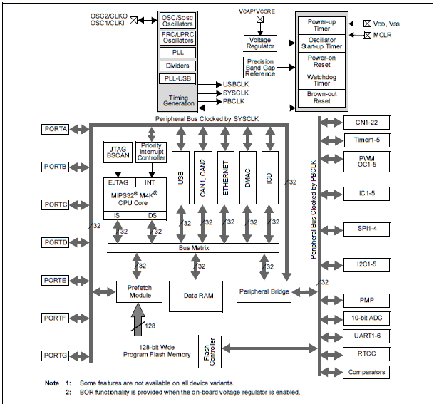
VI.2. Embedded devices, development environments for PCs
As we have seen so far, SOCs have less memory and storage device than PCs and they generally do not have a display device. Microcontrollers contain even less memory. Development environments made for these devices do not run on the given device (cannot even do so) but on a general purpose computer, which is normally a PC. The core of SOCs is generally some kind of a RISC processor. GCC is able to generate code for that in a cross-compiler mode. There is no frontend for the development tool: C source codes are written in a text editor and then they are compiled by the cross-compiler GCC. The Linux kernel, the system files as well as user files and a bootloader are put together in a ROM file and it is that whole file that is put in the EEPROM of the SOC. At the first time, when the bootloader is not yet present, the EEPROM can be written through the JTAG port of the SOC, with a JTAG burner. No SDK (software development kit) is normally made for SOCs because they are made by one-off production, therefore ICs are not sold individually but integrated in a device. For devices ready to be used (e.g. wide-band router) and if they use Linux, a source has to be provided on the website of the manufacturer. By modifying this, the functioning of the device can be intervened into or another Linux can be compiled for that device. An example for the latter is the OpenWRT project, in which a unique distribution was made by cross-gcc under Linux, and this can be loaded to routers mentioned in the documentation. OpenWRT is a relatively well documented project. Documentation was made by reverse-engineering, from the GPL source of the product.
In the case of microcontrollers, the situation is different. They are devices, produced in large quantities, without software and with general purposes, making it possible for users to write a program appropriate for the task. The language most frequently applied is K&R C. (Running a C++ code would require too much memory.) The smaller, 8-bit microcontrollers can be programmed in machine code as well. The advantage of the machine code is that it results in a small, efficient and fast program. Its disadvantage is that the code (and the knowledge about the instruction set) is not portable. Microcontroller manufacturers provide development tools in all cases: starting from the free compilers, intended to be used for an educational purpose (but already working and downloadable from the website of the manufacturer) to the professional development environments intended for companies. Other microcontrollers are supported by GCC as well. For these, the manufacturers provide only header files and front-ends. Since compilers compile files in C into executable ROM files as command line compilers, Visual Studio can also be used as a front-end when it is adequately set. The code ready to be used can be loaded into the microcontroller with JTAG or with a programmer of the given microcontroller. In general, contrary to the costly JTAG, these programmers can be bought at a price near 50$ and the Internet is full of circuit diagrams which may be used to get a useful solution for 1 or 2$.
In the following parts, the devices of the two largest microcontroller manufacturers, Atmel and Microchip, are presented. The two manufacturers produce more or less the same products: it's a matter of taste which one to choose. Atmel mostly aims at professional users, and this is reflected in the price, too. Microchip produces for beginners as well: a microcontroller with DIP socket to be soldered at home can be bought in small quantities as well (even one) from an official distributor in Hungary. Both manufacturer produce so-called starter-kits which contain a ready test panel with a microcontroller, input and output peripheral devices (in the cheaper version these are LEDs and buttons, in the more expensive version these are DC motors and touch screens), a programmer and demo-programs ready to be compiled and executed.
VI.2.1. Atmel: WinAVR and the AVR Studio
Most Atmel microcontrollers are supported by the GCC compiler as well, so an open-source IDE is available for them. The WinAVR can be found on the Sourceforge web page.. It can be downloaded free and without registration. After the installation the GCC compiler, and the necessary binutils and the gdb debugger can be used as well. Free programs generally do not have functionalities providing comfort or program libraries for special hardware elements: these have to be installed separately. The Figure VI.3, “The example program” shows the process of WinAVR's compilation of a sample program downloadable from the Internet that makes a LED flash. The files Makefile and led.c had to be written manually for that project in a text editor and then the "Make All” of the Tools menu had to be chosen.
The first two compiled value assignment statements:
void main(void)
{ unsigned char i;
// set PORTD for output
DDRB = 0xFF;
34: 8f ef ldi r24, 0xFF ; 255
36: 87 bb out 0x17, r24 ; 23
PORTB = 0b00000001;
38: 81 e0 ldi r24, 0x01 ; 1
3a: 88 bb out 0x18, r24 ; 24
The EEPROM content (led.eep) is now ready, and this can now be burnt into the ATTiny2313 with the avrdude programming utility and with an stk600 (200$) or with an AVRISP (40$) hardware.
Atmel also made its own IDE to which they provide many program libraries - this is called AVR Studio. It contains an integrated C compiler, but the actual Internet using society use the GCC compiler, so the AVR Studio can be configured in a way that it would work with the GCC compiler that can be found in WinAVR.
VI.2.2. Microchip: MPLAB IDE and MPLAB-X
At Microchip, there is no GCC support (although the picgcc project exists but it does not have a downloadable version), so the MPLAB IDE can be downloaded free from the website of the company. This contains an assembler compiler (MPASM) for all their products (16xx, 18xx, 24xx, dsPIC), with the exception of the Pic32 family (MIPS core:asm32), and it contains a C compiler with an education licence for the 18 (c18), 24 (c24) and 32 (c32) series. Besides editing, the the IDE supports all the available programmers and debuggers. If the IDE is intended to be used in a comfortable way, we should not accept "full installation", only the already existing (planned) devices and compilers should be installed. MPLAB SIM could be a useful tool with which programs can be executed and debugged without a concrete hardware, on a virtual CPU. The great advantage of a virtual CPU is that it cannot be ruined with a power supply of reversed polarity, contrary to real ones. The Figure VI.4, “The MPLAB IDE” shows the development of a program code that communicates with the (SerialPort) program that can be found in Section IV.2.23, “SerialPort”.
The code portion on Figure VI.4, “The MPLAB IDE” can be burnt into a PIC18f4550 with a PicKit2 (original: 40$, clone: 25$) and after that communication with the hardware is possible through USB.
The problems arising during the development of MPLAB IDE (dependency on Windows) are attempted to be solved in the new MPLAB-X. The NetBeans-based environment runs on both Linux and MacOS-X. This contains the automatic code completion functionality of the Visual Studio and the function definition finder.
VI.3. Programming of distributed systems
With the expansion of Internet and its base protocol, not only interpersonal communication accelerated a lot. Nowadays, supercomputers contain more than one processor with a big clock rate as well as big memories and data storage devices. The clock rate have reached the technological limit, an increase in performance can only be achieved by increasing the number of the basic computing components that can function parallelly in the same time. This can be achieved by encasing more processor cores within the same integrated circuit (Dual, Quad, etc. core).So it was a useful idea to share tasks on the Internet as well. The Internet connection between two machines takes place as a sequential file with the usage of socket software packages. The first method that is based on sockets but making possible an access on a higher level than sockets is remote procedure call (RPC), like that used in SUN NFS Unix-based file servers. However, programmers do not intend to develop protocols, error handling and file access. There are also object-oriented technologies as well that are based on sockets. In the case of these technologies, the properties of objects on a server are accessible on its clients; their methods can be run on servers as simple function calls on clients. Similarly, an event arising on a server can be handled with a triggered method on a client. It is also possible that only one proxy should be assigned to an IP-address and that it is the former that transfers a query of a user to a server computer that is free at that moment. Nowadays, systems with big computing needs work on a similar principle both in commerce and in education. This is the case for example for amazon.com, system of Google or JUQUEEN and JUROPA machines (IBM).
VI.3.1. CORBA
CORBA is a standardized object environment defined by OMG (Object Management Group). Its first version appeared in 1990 with which applications written in different languages and/or running on separate computers can work together. This application can use methods on the remote machines in the same way as on the local machines. An important element of the standard is interface definition language (IDL), which is independent of the actually used compiler (that may compile from C, C++, Java, Cobol and from some other languages). CORBA compilers make function headers (skeletons) for the objects written in IDL for the given language. These skeletons have to be implemented for the given language by programmers: this process is called "mapping". The objects made during this process are called "adapters". Mapping is easy in Java because of the strong object-oriented properties of that language. In C++, a little bit more work has to be carried out to achieve the same: complex data structures have to be used and these may sometimes become mixed with the types of Standard Template Library (STL). The CORBA implementation contains an IDL compiler that compiles to the used language (e.g. C++). An executable program can be created with an ordinary compiler and linker, of course by defining functions compiled from IDL (by "dressing" the skeletons) in the given language. Besides that, it contains native communication components which carry out communication on the Internet on the socket level in a way that is transparent to users. The Figure VI.5, “The structure of CORBA” demonstrates the access of an object operating on a server from a client.
VI.3.2. Open-source implementations of CORBA
CORBA is a standard so it cannot be obtained from a manufacturer: many people have implemented that structure. Among these, there are licensed (that can be bought) and open-source versions. The licensed ones are mainly widespread in the financial sector, open-source versions available for free are used for educational purposes.
MICO: www.mico.org contains only Unix API calls, written in C++, developed by the University of Frankfurt. Source files are stored on SourceForge, from where they can be downloaded
JacORB: www.jacorb.org, ORB written in Java, with an LGPL license. Needs JDK 1.6 to function.
TAO: www.ociweb.com, developed by the University of Washington, it has a free and a commercial version. Can be used both under Unix and Windows and there is also a version that runs under a real-time operating system.
ORBiT: orbit-resource.sourceforge.net can be used in basic C and Perl, an open-source CORBA 2.4 implementation. Since it was developed for GNOME system, most Linux distributions contain it. It has a version running under Win32.
The following example carries out a "remote" calculation: the client determines the operation, the server carries it out and then the client prints out the result. When tested, both the server-side and the client-side program run on the same computer. The IDL file is as simple as possible, it contains an interface with two functions:
// Calculator interface: calculator.idl
//
interface Calculator
{
double add(in double number1, in double number2);
double sub(in double number1, in double number2);
};
Let's compile it with the idl compiler: /usr/pkg/bin/orbit-idl-2 calculator.idl
orbit-idl-2 2.14.17 compiling mode, hide preprocessor errors, passes: stubs skels common headers Processing file calculator.idl
Now the skeleton (calculator-skel.c), the stub that can be executed on the client (calculator-stubs.c) and the headers (calculator.h) are generated. The header file contains a CORBA-compatible class (basic C with struct functions):
typedef struct {
void *_private;
CORBA_double (*add)(PortableServer_Servant _servant, const CORBA_double number1, const CORBA_double number2, CORBA_Environment *ev);
CORBA_double (*sub)(PortableServer_Servant _servant, const CORBA_double number1, const CORBA_double number2, CORBA_Environment *ev);
} POA_Calculator__epv;
These have to be implemented (skelimpl.c):
static CORBA_double
impl_Calculator_add(impl_POA_Calculator * servant,
const CORBA_double number1,
const CORBA_double number2, CORBA_Environment * ev)
{
CORBA_double retval;
/* ------ insert method code here ------ */
g_print ("%f + %f\n", number1, number2);
retval = number1 + number2;
/* ------ ---------- end ------------ ------ */
return retval;
}
static CORBA_double
impl_Calculator_sub(impl_POA_Calculator * servant,
const CORBA_double number1,
const CORBA_double number2, CORBA_Environment * ev)
{
CORBA_double retval;
/* ------ insert method code here ------ */
g_print ("%f - %f\n", number1, number2);
retval = number1 - number2;
/* ------ ---------- end ------------ ------ */
return retval;
}
Now the server-side main program can be the next:
static CORBA_Object
server_activate_service (CORBA_ORB orb,
PortableServer_POA poa,
CORBA_Environment *ev)
{
Calculator ref = CORBA_OBJECT_NIL;
ref = impl_Calculator__create (poa, ev);
if (etk_raised_exception(ev))
return CORBA_OBJECT_NIL;
return ref;
}
The service is started in the main() function of the server:
servant = server_activate_service (global_orb, root_poa, ev); server_run (global_orb, ev);
The stub does not have to be modified on the client, it is only the main() function that has to be written:
static
void
client_run (Calculator service,
CORBA_Environment *ev)
{
CORBA_double result=0.0;
result = Calculator_add(service, 1.0, 2.0, ev);
g_print("Result: 1.0 + 2.0 = %2.0f\n", result);
}
This is called from the main() function of the client and the server does the calculation:
./calculator-server the server is launched in the background, and it waits for the connection of the client
./calculator-client the client is started
1.000000 + 2.000000
Result: 1.0 + 2.0 = 3
VI.3.3. ICE – internet communication engine
Having examined the CORBA system, we have found that it can be applied to many tasks; however, most of the programming work has to be used for useless overcomplicated objects and classes. For that purpose, some CORBA developers created a little developer team to create a system supporting access of remote objects in a simplified (but in the same time) extended way by rethinking the principles of CORBA. For that purpose, they founded a company under the name ZeroC (www.zeroc.com). They named their system ICE, and it is available under two licences: GPL and commercial licence. The commercial version (for which we have to pay) comes with a product support. Another advantage of ICE is that it has a version running on touch-screen platforms that are popular nowadays, e.g. IceTouch, which was made for the compiler of OS-X (Xcode) and contains an iOS simulator, too.
The ICE distribution contains everything the environment needs: devices, APIs, libraries for the creation of object-oriented client-server applications. It supports the compatibility between architectures and languages: a client and a server can run under a different platform and the two may be written in other languages. The descriptor language in which an ICE object is defined is called Slice (Specification Language for Ice). It contains interfaces, operations and data types defined commonly on both the server and a client. These Slice files are compiled by a compiler to API calls, to code portions in different languages, which can be compiled on the currently used system and programming language, but of course only after skeletons are filled in (i.e. the portion between {} of functions are written). Compilation to a given language is called "language mapping". The language used in the Ice system can be C++, Java, C#, Python and Objective-C. The client-side can use PHP as well. The structure of programs using ICE can be seen in the Figure VI.6, “The structure of ICE programs”.
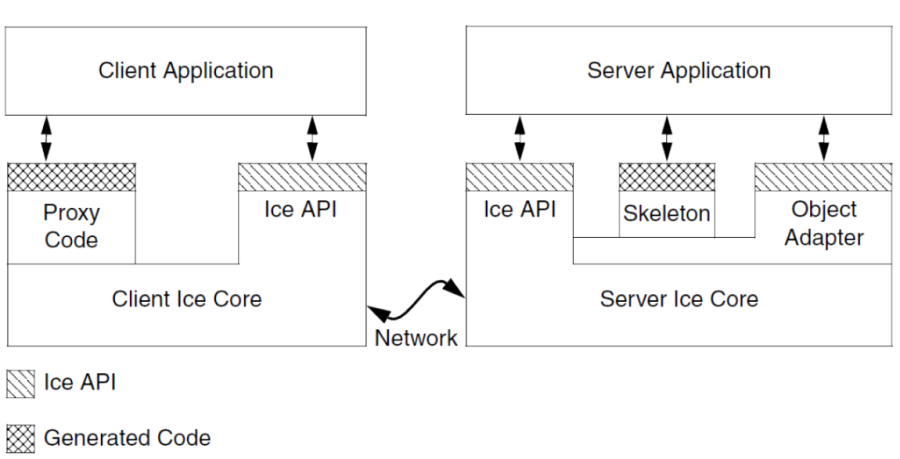
ICE uses its own protocol over IP: this may be TCP or UDP. If objects contain important data, SSL can also be used between servers and clients. Besides ordinary remote objects, it offers extra services, like IceGrid, in which more servers can contain the same object for the purpose of load-balancing; or IceStorm, which share events between publishers and subscribers interested in those events.
In the following simplified example, the ICE server-side of an industrial robot is created. The clients connected to the robot are able to move the robot and to obtain the actual coordinates. The slice definition file is the following (KukaRobot.ice – it can only be opened as a text file in the Visual Studio):
module CyberLab
{
struct e6pos
{
float x; // x,y,z are millimeters
float y;
float z;
float a; // a,b,c angles in degrees
float b;
float c;
};
interface Robot6Dof
{
void GotoHome(); // home position defined in robot program
e6pos GetPosition(); // where are you ?
void GotoPosition(e6pos p); // go to the position
};
};
When this file is compiled with slice2cpp.exe, 2 files are created: KukaRobot.cpp and KukaRobot.h. This is the so-called skeleton, in which the defined methods figure as abstract virtual member functions:
virtual void GotoPosition(const ::CyberLab::e6pos&, const ::Ice::Current& = ::Ice::Current()) = 0;
The last function of the interface can easily be recognized. In order to instantiate the class, we have to define this function. A new class (the implementation class: Robot6DofI) is derived from the class named Robot6Dof. This new class contains the implementation of these member functions – prototypes:
class Robot6DofI : public Robot6Dof {
public:
virtual void GotoHome(const Current& c);
virtual e6pos GetPosition(const Current& c);
virtual void GotoPosition(const e6pos& e6, const Current& c);
};
and defintions:
void Robot6DofI::GotoHome(const Current& c)
{
Send_command_to_robot(CMD_ROBOT_HOME);
}
e6pos Robot6DofI::GetPosition(const Current& c)
{
e6pos poz;
Send_command_to_robot(CMD_ROBOT_GET_POSITION,poz);
return poz;
}
void Robot6DofI::GotoPosition(const e6pos& e6, const Current& c)
{
Send_command_to_robot(CMD_ROBOT_GOTO_POSITION,e6);
}
When these functions were defined, we used the already existing communication functions that sent instructions through RS-232 with the robot. The last thing to be done is writing the main program and creating the communication adapter (on the basis of the ICE demo):
int _tmain(int argc, _TCHAR* argv[])
{
int status = 0;
std::string s1="KukaRobotAdapter";
std::string s2="default -p 10000";
Ice::CommunicatorPtr ic;
Ice::InitializationData id;
argc=0;
try
{
ic = Ice::initialize(id);
Ice::ObjectAdapterPtr adapter=ic->createObjectAdapterWithEndpoints
(s1,s2);
Ice::ObjectPtr object = new Robot6DofI;
adapter->add(object,ic->stringToIdentity("KukaRobot"));
adapter->activate();
ic->waitForShutdown();
}
catch (const Ice::Exception& e)
{
cerr << e << endl;
status = 1;
}
catch (const char* msg)
{
cerr << msg << endl;
status = 1;
}
if (ic)
{
try
{
ic->destroy();
}
catch (const Ice::Exception& e)
{
cerr << e << endl;
status = 1;
}
}
return status;
}
Do not forget about setting the ICE include and library directories in the Settings of the project because it is not able to compile and link the program without them.
When compilation has taken place correctly, the thing left to be done is making available the DLLs belonging to the ICE while the program runs and then starting the server. When the file named KukaRobot.ice is sent to the foreign partner, the latter creates the client (in a language, e.g. C#) and can control the robot remotely.
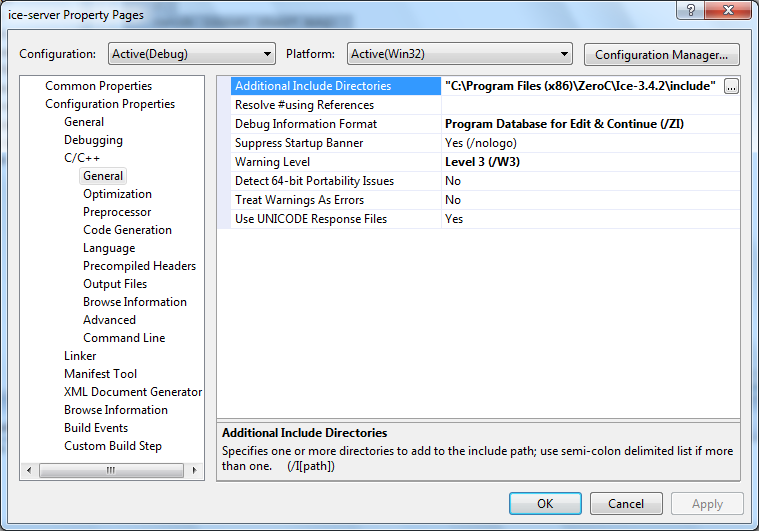
Appendix A. Appendix – Standard C++ summary tables
- A.1. ASCII code table
- A.2. Reserved keywords in C++
- A.3. Escape characters
- A.4. C++ data types and their range of values
- A.5. Statements in C++
- A.6. C++ preprocessor directives
- A.7. Precedence and associativity of C++ operations
- A.8. Some frequently used mathematical functions
- A.9. C++ storage classes
- A.10. Input/Output (I/O) manipulators
- A.11. The standard C++ library header files
A.1. ASCII code table
|
CHAR |
DEC |
HEX |
CHAR |
DEC |
HEX |
CHAR |
DEC |
HEX |
CHAR |
DEC |
HEX | |||
|---|---|---|---|---|---|---|---|---|---|---|---|---|---|---|
|
[NUL] |
0 |
00 |
32 |
20 |
@ |
64 |
40 |
` |
96 |
60 | ||||
|
[SOH] |
1 |
01 |
! |
33 |
21 |
A |
65 |
41 |
a |
97 |
61 | |||
|
[STX] |
2 |
02 |
" |
34 |
22 |
B |
66 |
42 |
b |
98 |
62 | |||
|
[ETX] |
3 |
03 |
# |
35 |
23 |
C |
67 |
43 |
c |
99 |
63 | |||
|
[EOT] |
4 |
04 |
$ |
36 |
24 |
D |
68 |
44 |
d |
100 |
64 | |||
|
[ENQ] |
5 |
05 |
% |
37 |
25 |
E |
69 |
45 |
e |
101 |
65 | |||
|
[ACK] |
6 |
06 |
& |
38 |
26 |
F |
70 |
46 |
f |
102 |
66 | |||
|
[BEL] |
7 |
07 |
' |
39 |
27 |
G |
71 |
47 |
g |
103 |
67 | |||
|
[BS] |
8 |
08 |
( |
40 |
28 |
H |
72 |
48 |
h |
104 |
68 | |||
|
[HT] |
9 |
09 |
) |
41 |
29 |
I |
73 |
49 |
i |
105 |
69 | |||
|
[LF] |
10 |
0A |
* |
42 |
2A |
J |
74 |
4A |
j |
106 |
6A | |||
|
[VT] |
11 |
0B |
+ |
43 |
2B |
K |
75 |
4B |
k |
107 |
6B | |||
|
[FF] |
12 |
0C |
, |
44 |
2C |
L |
76 |
4C |
l |
108 |
6C | |||
|
[CR] |
13 |
0D |
- |
45 |
2D |
M |
77 |
4D |
m |
109 |
6D | |||
|
[SO] |
14 |
0E |
. |
46 |
2E |
N |
78 |
4E |
n |
110 |
6E | |||
|
[SI] |
15 |
0F |
/ |
47 |
2F |
O |
79 |
4F |
o |
111 |
6F | |||
|
[DLE] |
16 |
10 |
0 |
48 |
30 |
P |
80 |
50 |
p |
112 |
70 | |||
|
[DC1] |
17 |
11 |
1 |
49 |
31 |
Q |
81 |
51 |
q |
113 |
71 | |||
|
[DC2] |
18 |
12 |
2 |
50 |
32 |
R |
82 |
52 |
r |
114 |
72 | |||
|
[DC3] |
19 |
13 |
3 |
51 |
33 |
S |
83 |
53 |
s |
115 |
73 | |||
|
[DC4] |
20 |
14 |
4 |
52 |
34 |
T |
84 |
54 |
t |
116 |
74 | |||
|
[NAK] |
21 |
15 |
5 |
53 |
35 |
U |
85 |
55 |
u |
117 |
75 | |||
|
[SYN] |
22 |
16 |
6 |
54 |
36 |
V |
86 |
56 |
v |
118 |
76 | |||
|
[ETB] |
23 |
17 |
7 |
55 |
37 |
W |
87 |
57 |
w |
119 |
77 | |||
|
[CAN] |
24 |
18 |
8 |
56 |
38 |
X |
88 |
58 |
x |
120 |
78 | |||
|
[EM] |
25 |
19 |
9 |
57 |
39 |
Y |
89 |
59 |
y |
121 |
79 | |||
|
[SUB] |
26 |
1A |
: |
58 |
3A |
Z |
90 |
5A |
z |
122 |
7A | |||
|
[ESC] |
27 |
1B |
; |
59 |
3B |
[ |
91 |
5B |
{ |
123 |
7B | |||
|
[FS] |
28 |
1C |
< |
60 |
3C |
\ |
92 |
5C |
| |
124 |
7C | |||
|
[GS] |
29 |
1D |
= |
61 |
3D |
] |
93 |
5D |
} |
125 |
7D | |||
|
[RS] |
30 |
1E |
> |
62 |
3E |
^ |
94 |
5E |
~ |
126 |
7E | |||
|
[US] |
31 |
1F |
? |
63 |
3F |
_ |
95 |
5F |
[DEL] |
127 |
7F |
A.2. Reserved keywords in C++
|
and |
double |
not |
this |
|
and_eq |
dynamic_cast |
not_eq |
throw |
|
asm |
else |
operator |
true |
|
auto |
enum |
or |
try |
|
bitand |
explicit |
or_eq |
typedef |
|
bitor |
export |
private |
typeid |
|
bool |
extern |
protected |
typename |
|
break |
false |
public |
union |
|
case |
float |
register |
unsigned |
|
catch |
for |
reinterpret_cast |
using |
|
char |
friend |
return |
virtual |
|
class |
goto |
short |
void |
|
compl |
if |
signed |
volatile |
|
const |
inline |
sizeof |
wchar_t |
|
const_cast |
int |
static |
while |
|
continue |
long |
static_cast |
xor |
|
default |
mutable |
struct |
xor_eq |
|
delete |
namespace |
switch | |
|
do |
new |
template |
In the 1998 ANSI/ISO C++ standard
|
alignas |
char32_t |
final |
override |
|
alignof |
constexpr |
noexcept |
static_assert |
|
char16_t |
decltype |
nullptr |
thread_local |
Additional keywords added by the C++11 standard
A.3. Escape characters
|
Description |
ASCII character |
Escape sequence |
|---|---|---|
|
audible bell (alert) |
BEL |
'\a' |
|
backspace |
BS |
'\b' |
|
form feed – new page |
FF |
'\f' |
|
line feed - new line |
NL (LF) |
'\n' |
|
carriage return |
CR |
'\r' |
|
horizontal tab |
HT |
'\t' |
|
vertical tab |
VT |
'\v' |
|
single quote |
' |
'\'' |
|
double quote |
" |
'\"' |
|
backslash |
\ |
'\\' |
|
question mark |
? |
'\?' |
|
ANSI character with an octal code |
ooo |
'\ooo' |
|
Null character |
NUL |
'\0' |
|
ANSI character with a hexadecimal code |
hh |
'\xhh' |
|
16-bit Unicode character |
hhhh |
'\uhhhh' |
|
32-bit Unicode character |
hhhhhhhh |
'\Uhhhhhhhh' |
A.4. C++ data types and their range of values
|
Data type |
Range of values |
Size (bytes) |
Precision (digits) |
|---|---|---|---|
|
bool |
false, true |
1 | |
|
char |
-128..127 |
1 | |
|
signed char |
-128..127 |
1 | |
|
unsigned char |
0..255 |
1 | |
|
wchar_t |
0..65535 |
2 | |
|
int |
-2147483648..2147483647 |
4 | |
|
unsigned int |
0..4294967295 |
4 | |
|
short |
-32768..32767 |
2 | |
|
unsigned short |
0..65535 |
2 | |
|
long |
-2147483648..2147483647 |
4 | |
|
unsigned long |
0..4294967295 |
4 | |
|
long long |
-9223372036854775808.. 9223372036854775807 |
8 | |
|
unsigned long long |
0..18446744073709551615 |
8 | |
|
float |
3.4E-38..3.8E+38 |
4 |
6 |
|
double |
1.7E-308..1.7E+308 |
8 |
15 |
|
long double |
3.4E-4932..3.4E+4932 |
10 |
19 |
A.5. Statements in C++
|
Category |
C++ statements |
|---|---|
|
Declaration/definition statements |
types (class, struct, union, enum, typedef), functions, objects |
|
Expression statements |
expression; |
|
Empty statement |
; |
|
Compound statement |
{ statements } |
|
Selection statements |
if, else,switch, case |
|
Iteration statements |
do, for, while |
|
Flow control statements |
break, continue, default, goto, return |
|
Exception handling statements |
throw, try-catch |
A.6. C++ preprocessor directives
|
Category |
Directive |
|---|---|
|
Conditional directive |
#ifdef, #ifndef, #if, #endif, #else, #elif |
|
Defining symbols/macros |
#define |
|
Undefining symbols/macros |
#undef |
|
Including source files |
#include |
|
Generating compilation errors |
#error |
|
Modifying the line number (and file name) in compilation messages |
#line |
|
Implementation dependent control of the compilation process |
#pragma |
Predefined macros
|
Macro |
Description |
|---|---|
|
|
String containing the date of the compilation. |
|
|
String containing the time of the compilation. |
|
|
String containing the name of the source file. |
|
|
A numeric constant containing the actual line number of the source file (numbering starts from 1). |
|
|
Its value is 1 if the compiler works as an ANSI C++ compiler, otherwise it is not defined. |
|
|
Its value is 1, if in a C++ source file, otherwise it is not defined. |
|
|
Its value is 1, if in a C++/CLI source file, otherwise it is not defined. |
A.7. Precedence and associativity of C++ operations
|
Precedence |
Operator |
Name or meaning |
Associativity |
|---|---|---|---|
|
1. |
:: |
scope resolution |
none |
|
2. |
( ) |
function call, member initialization |
from left to right |
|
[ ] |
array indexing | ||
|
-> |
indirect member selection (pointer) | ||
|
. |
direct member selection (object) | ||
|
++ |
(postfix) increment | ||
|
-- |
(postfix) decrement | ||
|
type () |
type-cast (conversion) | ||
|
dynamic_cast |
checked type-cast at runtime (conversion) | ||
|
static_cast |
checked type-cast during compilation time (conversion) | ||
|
reinterpret_cast |
unchecked type-cast (conversion) | ||
|
const_cast |
constant type-cast (conversion) | ||
|
typeid |
type identification | ||
|
3. |
! |
logical negation (NOT) |
from right to left |
|
~ |
bitwise negation | ||
|
+ |
+ sign (numbers) | ||
|
- |
- sign (numbers) | ||
|
++ |
(prefix) increment | ||
|
-- |
(prefix) decrement | ||
|
& |
address-of operator | ||
|
* |
indirection operator | ||
|
( type ) |
type-cast (conversion) | ||
|
sizeof |
size of an object/type in bytes | ||
|
new |
allocating dynamic memory space | ||
|
delete |
deallocating dynamic memory space | ||
|
4. |
.* |
direct reference to a class member |
from left to right |
|
->* |
indirect reference to a member of the object the pointer points to | ||
|
5. |
* |
multiplication |
from left to right |
|
/ |
division | ||
|
% |
modulo | ||
|
6. |
+ |
addition |
from left to right |
|
– |
subtraction | ||
|
7. |
<< |
bitwise left shift |
from left to right |
|
>> |
bitwise right shift | ||
|
8. |
< |
less than |
from left to right |
|
<= |
less than or equals | ||
|
> |
greater than | ||
|
>= |
greater than or equals | ||
|
9. |
== |
equal to |
from left to right |
|
!= |
not equal to | ||
|
10. |
& |
bitwise AND |
from left to right |
|
11. |
| |
bitwise inclusive OR |
from left to right |
|
12. |
^ |
bitwise exclusive OR (XOR) |
from left to right |
|
13. |
&& |
logical AND |
from left to right |
|
14. |
|| |
logical OR |
from left to right |
|
15. |
expr ? expr : expr |
conditional expression |
from right to left |
|
16. |
= |
simple value assignment |
from right to left |
|
*= |
multiplication assignment | ||
|
/= |
division assignment | ||
|
%= |
modulo assignment | ||
|
+= |
addition assignment | ||
|
-= |
subtraction assignment | ||
|
<<= |
bitwise left shift assignment | ||
|
>>= |
bitwise right shift t assignment | ||
|
&= |
bitwise AND assignment | ||
|
^= |
bitwise XOR assignment | ||
|
|= |
bitwise OR assignment | ||
|
17. |
throw expr |
throwing an expression |
from right to left |
|
18. |
expr , expr |
operation sequence (comma operator) |
from left to right |
A.8. Some frequently used mathematical functions
|
Usage |
Type |
Function |
Include file |
|---|---|---|---|
|
calculation of absolute value |
real |
|
|
|
calculation of absolute value |
integer |
|
|
|
cosine of an angle (in radians) |
real |
|
|
|
sine of an angle (in radians) |
real |
|
|
|
tangent of an angle (in radians) |
real |
|
|
|
the inverse cosine of the argument (in radians) |
real |
|
|
|
the inverse sine of the argument (in radians) |
real |
|
|
|
the inverse tangent of the argument (in radians) |
real |
|
|
|
the inverse tangent of y/x (in radians) |
real |
|
|
|
natural logarithm |
real |
|
|
|
base 10 logarithm |
real |
|
|
|
ex |
real |
|
|
|
power (xy) |
real |
|
|
|
square root |
real |
|
|
|
random number between 0 and RAND_MAX |
real |
|
|
|
the value of π |
real |
|
|
Where the type real designates one of the following types: float, double or long double. The type integer designates one of the int or long types
A.9. C++ storage classes
|
Properties |
Result | |||
|---|---|---|---|---|
|
Scope |
Item |
Storage class |
Lifetime |
Visibility |
|
file-level |
variable definition |
|
global |
restricted to a given file, from its definition to the end of the file |
|
variable declaration |
|
global |
from its definition to the end of the file | |
|
prototype or function definition |
|
global |
restricted to the given file | |
|
function prototype |
|
global |
from its definition to the end of the file | |
|
block-level |
variable declaration |
|
global |
block |
|
variable definition |
|
global |
block | |
|
variable definition |
|
local |
block | |
|
variable definition |
|
local |
block | |
A.10. Input/Output (I/O) manipulators
Parameterless manipulators <iostream>
The following manipulators are used in pairs, they have their effects from the time they are set until they are unset:
|
Manipulator |
Stream |
Description (when they are set) |
|---|---|---|
|
|
I/O |
The logical values can be provided with the keywords true and false. |
|
|
O |
The sign of the numeral system is also printed out before numbers (0 or 0x). |
|
|
O |
Decimal point is always printed. |
|
|
O |
A plus sign always printed out for any number that is not negative. |
|
|
I |
Discarding whitespace characters. |
|
|
O |
Flushing the buffer automatically after each operation. |
|
|
O |
When numbers are printed out, (e and x) will always be uppercase |
Some manipulators modifying data streams:
|
Manipulator |
Stream |
Description |
|---|---|---|
|
|
O |
Insert newline and flush. |
|
|
O |
Insert null character. |
|
|
O |
Flush the stream buffer. |
|
|
I |
Extract whitespaces. |
The effects of the following manipulators can be modified by those provided in the same group:
|
Manipulator |
Stream |
Description |
|---|---|---|
|
Alignment | ||
|
|
O |
Left-aligned |
|
|
O |
Right-aligned - default |
|
|
O |
The output is padded to the field as best as possible by inserting filler characters |
|
Numeral system | ||
|
|
I/O |
Decimal - default |
|
|
I/O |
Hexadecimal |
|
|
I/O |
Octal |
|
Printing out real numbers (if these manipulator flags are not set, the compiler decides their format) | ||
|
|
O |
Fixed-point notation |
|
|
O |
Scientific notation |
Parameterized manipulators <iomanip>:
setw affects only the data element that immediately follows him, and the others affect all subsequent data elements for the output stream.
|
Manipulator |
Stream |
Description |
|---|---|---|
|
|
O |
Set fill character. |
|
|
O |
Set decimal precision. |
|
|
O |
Set field width. |
|
|
O |
Sets the numeric base field (8,10,16). |
A.11. The standard C++ library header files
|
C++ language library | |
|
Types (NULL, size_t etc.) |
<cstddef> |
|
Limits of different types |
<limits>, <climits>, <cfloat> |
|
Program control |
<cstdlib> |
|
Dynamic memory handling |
<new> |
|
Type identification |
<typeinfo>, <typeindex>, <type_traits> |
|
Exception handling types |
<exception> |
|
Other run-time support |
<cstdarg>, <csetjmp>, <ctime>, <csignal>, <cstdlib>,<cstdbool>, <cstdalign> |
|
Diagnostic library | |
|
Exception classes |
<stdexcept> |
|
Assert macros |
<cassert> |
|
Error codes |
<cerrno> |
|
System error support |
<system_error> |
|
Library of general services | |
|
Function elements (STL) |
<utility> |
|
Function objects (STL) |
<functional> |
|
High level memory handling (STL) |
<memory>, <scoped_allocator> |
|
Special class templates (STL) |
<bitset>, <tuple> |
|
Date and time handling |
<ctime> , <chrono> |
|
String library | |
|
String classes |
<string> |
|
C-style string handling |
<cctype>, <cwctype>, <cstring>, <cwchar>, <cstdlib>, <cuchar> |
|
Library of country-specific (local) settings | |
|
Localization utilities |
<locale> |
|
C localization utilities |
<clocale> |
|
Unicode conversion facilities |
<codecvt> |
|
Library of containers (STL) | |
|
Sequential containers (STL) |
<array>, <deque>, <list>, <vector>, <forward_list> |
|
Associative containers (STL) |
<map>, <set> |
|
Unordered associative containers(STL) |
<unordered _map>, <unordered_set> |
|
Container adaptors (STL) |
<queue>, <stack> |
|
Library of iterators (generic pointers) (STL) | |
|
Iterator elements, predefined iterators, data stream iterators (STL) |
<iterator> |
|
Algorithms library | |
|
Algorithms that operate on containers (STL) |
<algorithm> |
|
Algorithms of the C library |
<cstdlib> |
|
Numeric library | |
|
Complex number type |
<complex> |
|
Representing and manipulating arrays of values |
<valarray> |
|
Numeric operations on values in containers |
<numeric> |
|
The numeric elements of the C library |
<cmath>, <cstdlib>, <ctgmath> |
|
Compile-time rational arithmetic |
<ratio> |
|
Random number generators and distributions |
<random> |
|
Floating-point environment access functions |
<cfenv> |
|
Standard Input/Output library | |
|
Forward declarations of all I/O classes |
<iosfwd> |
|
Standard iostream objects |
<iostream> |
|
The base class of the iostream classes |
<ios> |
|
Data stream buffers |
<streambuf> |
|
Data formatting and manipulators |
<istream>, <ostream>, <iomanip> |
|
String data streams |
<sstream> |
|
File data streams |
<fstream>, <cstdio>, <cinttypes> |
|
Regular expressions library | |
|
Regular expression processing. |
<regex> |
|
Functions for concurrent programming | |
|
Atomic types and operations |
<atomic> |
|
Thread support library | |
|
Creating and controlling threads |
<thread>, <mutex>, <condition_variable>, <future> |
The underscored names are the header files of the C++11 standard.
Appendix B. Appendix – C++/CLI summary tables
B.1. C++/CLI reserved words
|
|
|
|
|
|
|
|
|
|
|
|
|
|
|
|
|
|
|
|
|
|
|
|
|
|
|
|
|
B.2. The types of classes and structures in C++/CLI
|
Keyword |
Domain |
Default access |
Equivalent |
Used by |
|---|---|---|---|---|
|
|
native |
private |
class in C++ |
value, native pointer or reference |
|
|
native |
public |
struct in C++ |
value, native pointer or reference |
|
|
managed |
private |
class in C# |
managed reference |
|
|
managed |
public |
class in C# |
managed reference |
|
|
managed |
private |
struct in C# |
value |
|
|
managed |
public |
struct in C# |
value |
B.3. Operators for pointers and references in C++/CLI
|
Operation |
Native Code |
Managed Code |
|---|---|---|
|
Pointer definition Pointer dereference |
* |
^ |
|
Reference definition Address-of |
& |
% |
|
Member access |
-> |
-> |
|
Allocation |
new |
gcnew |
|
Deallocation |
delete |
delete (calls Dispose) |
B.4. The .NET (CTS) and the C++/CLI primitive types
|
.NET type |
C++/CLI |
|---|---|
|
Char |
wchar_t |
|
Boolean |
bool |
|
Byte |
unsigned char |
|
SByte |
char |
|
Int16 |
short |
|
UInt16 |
unsigned short |
|
Int32 |
int, long |
|
UInt32 |
unsigned int, unsigned long |
|
Int64 |
long long |
|
UInt64 |
unsigned long long |
|
Double |
double |
|
Single |
float |