Chapter 4. Sliding mode control
Prev		Next

Chapter 4. Sliding mode control

Table of Contents

4.1. Short historical overview

The sliding mode control has a unique place in control theories. First, the exact mathematical treatment represents numerous interesting challenges for the mathematicians. Secondly, in many cases it can be relatively easy to apply without a deeper understanding of its strong mathematical background and is therefore widely used in engineering practice. This article is intended to constitute a bridge between the exact mathematical description and the engineering applications. After a short overview of the sliding mode control the article presents its mathematical foundations, namely the theory of differential equations with discontinuous right-hand sides. The power electronic circuits, which always have some kind of switching elements, can be typically described by such differential equation. Such equations don’t fulfill the regular theorem of existence and uniqueness, but under certain conditions remain valid, if we interpret the solution of the differential equation according to the definition proposed by Filippov. The article presents a practical example of the definition proposed by Filippov per a sliding mode control of an L-C circuit and an experimental application on uninterruptible power supply.

Recently most of the controlled systems are driven by electricity as it is one of the cleanest and easiest (with smallest time constant) to change (controllable) energy source. The conversion of electrical energy is solved by power electronics. One of the most characteristic common features of the power electronic devices is the switching mode. We can switch on and off the semiconductor elements of the power electronic devices in order to reduce losses because if the voltage or current of the switching element is nearly zero, then the loss is also near to zero. Thus, the power electronic devices belong typically to the group of variable structure systems (VSS). The variable structure systems have some interesting characteristics in control theory. A VSS might also be asymptotically stable if all the elements of the VSS are unstable itself. Another important feature that a VSS - with appropriate controller - may get in a state in which the dynamics of the system can be described by a differential equation with lower degree of freedom than the original one. In this state the system is theoretically completely independent of changing certain parameters and of the effects of certain external disturbances (e.g. non-linear load). This state is called sliding mode and the control based on this is called sliding mode control which has a very important role in the control of power electronic devices.

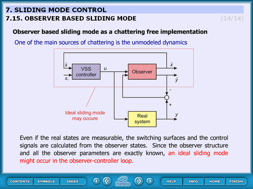
The theory of variable structure system and sliding mode has been developed decades ago in the Soviet Union. The theory was mainly developed by Vadim I. Utkin [1] and David K. Young [2]. According to the theory sliding mode control should be robust, but experiments show that it has serious limitations. The main problem by applying the sliding mode is the high frequency oscillation around the sliding surface, the so-called chattering, which strongly reduces the control performance. Only few could implement in practice the robust behavior predicted by the theory. Many have concluded that the presence of chattering makes sliding mode control a good theory game, which is not applicable in practice. In the next period the researchers invested most of their energy in chattering free applications, developing numerous solutions.

After the introduction, the second section summarizes the mathematical foundations of sliding mode control based on the theory of the differential equations with discontinuous right-hand sides, explaining how it might be applied for control relay. The third section shows how to apply the mathematical foundations on a practical example.

4.2. Introductory example

The first example introduces a problem that can often be found in the engineering practice. Assume that there is a serial L-C circuit with ideal elements, which can be shorted, or can be connected to the battery voltage by a transistor switch (see Figure 4-1., where the details of the transistor switch are not shown). Assume that our reference signal has a significantly lower frequency than the switching frequency of the controller. Thus we can take the reference signal as constant.

Figure 4.1. L-C circuit

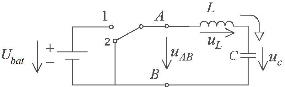
Assume that we start from an energy free state, and our goal is to load the capacitor to the half of the battery voltage by switching the transistor. The differential equations for the circuit elements are:

$C \frac{d}{d t} u_{c} = i_{c}$ and $L \frac{d}{d t} i_{L} = u_{L}$

(4.1)

Due to the serial connection ic = iL, thus the differential equation describing the system is:

$u_{A B} = u_{c} + L C \frac{d^{2}}{d t^{2}} u_{c}$

(4.2)

Introduce relative units such way, that LC = 1 and Ubat = 1. Introduce the error signal voltage ue = Ur - uc, where Ur = 1/2 is the reference voltage of the capacitor. Thus, the differential equation of the error signal has the form:

$u = u_{e} + \frac{d^{2}}{d t^{2}} u_{e}$ $, w h e r e$ $u = {\begin{matrix} \frac{1}{2}, if the switch is in state 1 \\ - \frac{1}{2}, if the switch is in state 2 \end{matrix}$

(4.3)

It is easy to see that the state belonging to the solution of (4.3) equation moves always clockwise along a circle on the phase plane $u_{e}, \frac{d}{d t} u_{e}$ (see Figure 4-2.).

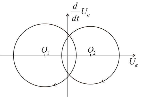
Figure 4.2. Possible state-trajectories.

The center of the circle depends on the state of the transistor. The state-trajectory is continuous, so the radius of the circle depends on in what state the system is at the moment of the last switching. Assume that we start from the state

$u_{e} = 1 / 2, \frac{d}{d t} u_{e} = 0$

(4.4)

and our goal is to reach by appropriate switching the state

$u_{e} = 0, \frac{d}{d t} u_{e} = 0$

(4.5)

Introduce the following switching strategy:

$u = \frac{1}{2} sign(s)$

(4.6)

where

(4.7)

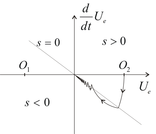
This means that if the state-trajectory is over the s = 0 line, then we have to switch the circle centered at O1, if it is below the line, then we have to switch the circle centered at O2. Examine how we can remove the error. Consider Figure 4-3., according to (4.6) and (4.7)(4.4) at first we start over the s = 0 line on a circle centered at O1. Reaching the line we switch to the circle centered at O2 so that the state-trajectory remains continuous. After the second switching we experience an interesting phenomenon. As the state trajectory starts along the circle centered at O1, it returns immediately into the area, where the circle centered at the O2 has to be switched, but the state-trajectory can not stay on this circle either, new switching is needed. For the sake of representation, the state-trajectory in Figure 4-3.reaches significantly over to the areas on both sides of the s = 0 line. In ideal case the state trajectory follows the s = 0 line on a curve broken in each points consisting of infinitely short sections switched by infinitely high frequency. In other words, the trajectory of the error signal slides along the s = 0 line and therefore is called sliding mode.

Figure 4.3. Removing the error.

Based on the engineering and geometric approach we feel that after the second switching, the behavior of the error signal can be described by the following differential equation instead of the second order (4.3):

$0 = u_{e} + λ \frac{d}{d t} u_{e}$

(4.8)

This is particularly interesting because (4.8) does not include any parameter of the original system, but the $λ$ we have given. Thus we got a robust control that by certain conditions is insensitive to certain disturbances and parameter changes. Without attempting to be comprehensive investigate the possible effects of changing some attributes and parameters of the system. If we substitute the ideal lossless elements by real lossy elements, then the state-trajectory instead of a circle moves along a spiral with decreasing radius. If the battery voltage fluctuates, the center of the circle wanders. Both changes affect the section before the sliding mode and modifies the sustainability conditions of the sliding mode, but in either case, the sliding mode may persist (the state trajectory can not leave the switch line), and if it persists, then these changes will not affect the behavior of the sliding mode of the system.

The next section will discuss how we can prove our conjecture mathematically.

4.3. Solution of differential equations with discontinuous right-hand sides

Consider the following autonomous differential equation system:

$\frac{d}{d t} x (t) = f (x (t))$ and $x (t = T_{0}) = X_{0}$

(4.9)

where

$x \in ℜ^{n}$ and $f (x) : ℜ^{n} \to ℜ^{n}$

(4.10)

If f(x) is continuous then we can write (4.5) as the integral equation:

(4.11)

The approach of (4.9) according to (4.11) is called Carathéodory solution, which under certain conditions may also exist when f(x) is discontinuous . Recently, several articles and PhD theses dealt with it how to ease the preconditions which guarantee the existence of (4.11) concerning f(x), but for the introduced example none of the cases might be applied, we need a completely different solution.

Filippov recommends a solution, which is perhaps closer to the engineering approach described in the previous section [3] [4]. Filippov is searching the solution of (4.9) at a given point based on how the derivative behaves in the neighborhood of the given point, allowing even that the behavior of the derivative may completely different from its neighborhood on a zero set, and regarding the solution ignores the derivative on this set. Filippov’s original definition concerns non-autonomous differential equations, but this article deals only with autonomous differential equations.

Consider (4.9) and assume that f(x) is defined almost everywhere on an open subset of $ℜ^{n}$ . Assume also that f(x) is measurable, locally bounded and discontinuous. Define the set K(x) for x $\subset$ f(x) by:

$K (x) : = \underset{δ > 0}{\cap} \underset{μ N = 0}{\cap} conv f (Q (x, δ) - N)$

(4.12)

where $Q (x, δ)$ denotes the open hull with center x and the radius , is the Lebesgue measure, N is the Lebesgue null set and the word "conv" denotes the convex closure of the given set.

Filippov introduced the following definition to solve the discontinuous differential equation systems:

Definition:

An absolutely continuous vector-valued function $x (t) : [T_{0}, T_{2}] \to G \in ℜ^{n}$ is the solution of (4.9) if

$\frac{d}{d t} x \subset K (x (t))$

(4.13)

for almost every $t \subset [T_{0}, T_{2}]$ . Note that if f(x) is continuous, then set K(x) has a single element for every x, namely f(x), thus the definition of Filippov is consistent with the usual differential equations (with continuous right-hand side). However, if f(x) is not continuous, then this definition allows us searching a solution for (4.9) in such a domain of x, where f(x) is not defined.

4.4. Control relays

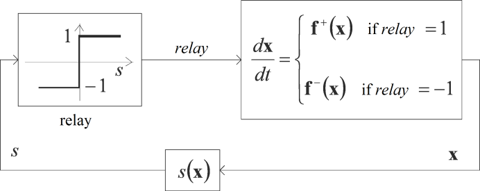
Apply the definition of Filippov as a generalization of the introductory example in the case of such a controller with state feedback, where in the feedback loop only a relay can be found (see ???

Figure 4-4.). Assume that the state of the system can be described by the differential equation (4.9), where the vectorfunction f(x) is standing on the right-hand side rapidly varies depending on the state of the relay. The control (switching) strategy should be the following. In the domain of the space $G \in ℜ^{n}$ defined by the fedback state variables define an n-1 dimensional smooth regular hypersurface S (which can also be called as switching surface) using continuous $s (x) : ℜ^{n} \to ℜ$ scalar-vector function in the following way:

Figure 4.4. Controller with relay

$S : = {x : s (x) = 0}$

(4.14)

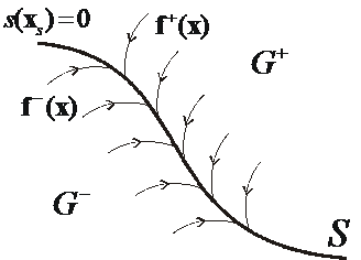
The goal of the controller is to force the state-trajectory to this surface. Mark the points of the surface S with xs. With the help of this surface we can divide the domain G into two parts:

$G^{+} : = {x : s (x) > 0}$	( 4.15 )
$G^{-} : = {x : s (x) < 0}$	( 4.16 )

Let the differential equation for x on domain G and our switching strategy have the following form:

$\frac{d}{d t} x = f (x) = {\begin{matrix} f^{+} (x), if x \in G^{+} \\ f^{-} (x), if x \in G^{-} \end{matrix}$

( 4.17 )

where f +(x) and f -(x) are uniformly continuous vector-vector functions.

Note that f(x) is not defined on the surface S, and we did not specify that f +(x) and f -(x) must be equal on both sides of the surface S.

Outside the surface S we have to deal with an ordinary differential equation. Solution of (4.17) might be a problem in the xs(t) points of the surface S. According to definition (4.13), K is the smallest closed convex set, which you get in the following way: let’s take an arbitrary $δ > 0$ hull of all xs(t) points of the xs belonging to the surface S, exclude f(xs), where f(x) is not defined (remark: it is a null set N domain), and we complete the set of f(x) vectors belonging to the resulting set to a closed convex set. Obviously, the smaller the value of $δ > 0$ , the smaller the resulting closed convex set. Finally, we need to take the intersection of the closed convex sets in the hull of all $δ > 0$ and N. Since f(x) is absolutely continuous, the following limits exist at any point of the surface S:

$\begin{matrix} \lim_{x \to x_{s}} f (x) = f^{+} (x_{S}) if x \in G^{+} \\ \lim_{x \to x_{s}} f (x) = f^{-} (x_{S}) if x \in G^{-} \end{matrix}$

(4.18)

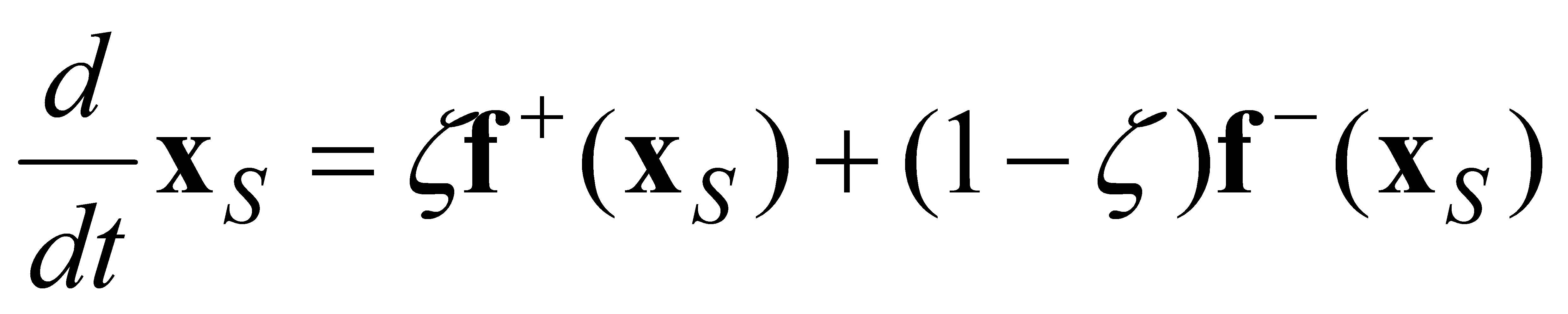
It means that the $\underset{δ > 0}{\cap} \underset{μ N = 0}{\cap} f (Q (x, δ) - N)$ set belonging to any point xs(t) of the surface S has only two elements, f +(xs) and f -(xs). We have to take the convex closure of these two vectors, which will be the smallest subset belonging to all $δ > 0$ values. In summary, the differential equation (4.9) with a (4.14) form discontinuity in the xs(t) points of S surface according to definition (4.13) can be described in the following form:

(4.19)

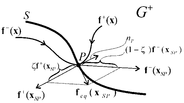
To illustrate (4.19) see ???

Figure 4-5., where we drew f +(xSP) and f -(xSP) vectors belonging to the point P of surface S. We marked the normal vector belonging to the point P of the surface with np. The change of the state trajectory in point xSP is given by the equivalent vector feq(xSP), which is the convex sum of vectors f +(xSP) and f -(xSP).

Figure 4.5. The state trajectory sliding along the surface S

Denote by Lfs(x) the directional derivative of the scalar function s(x) concerning the vector space f(x):

$L_{f} s (x) = (f (x) • grad(s (x)))$

(4.20)

where (a ● b) denotes the scalar product of vectors a and b. Since s(x) is uniformly continuous, the following limits exist at any point of the surface S:

$\begin{matrix} \lim_{x \to x_{s}} L_{f} s (x) = L_{f^{+}} s (x_{S}) if x \in G^{+} \\ \lim_{x \to x_{s}} L_{f} s (x) = L_{f^{-}} s (x_{S}) if x \in G^{-} \end{matrix}$

(4.21)

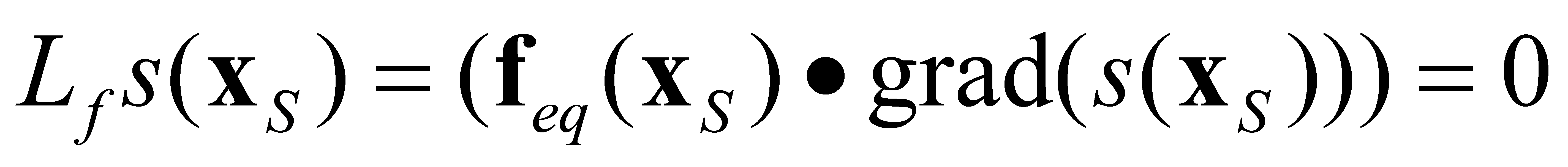
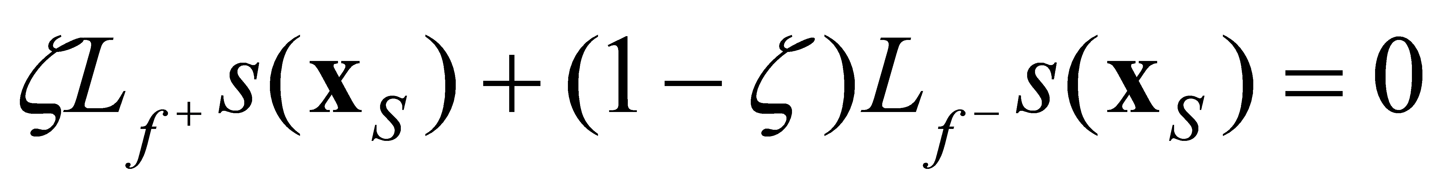
The value of should be defined such that $\frac{d}{d t} x_{S}$ and feq(xS) are orthogonal to the normal vector of the surface S (see Filippov 3. Lemma [3]):

(4.22)

The equation (4.22) can be interpreted in the following way: in sliding mode, in the xs points of the sliding surface the change of the state trajectory can be described by an equivalent feq(xS) vector function that satisfies condition(4.22). Based on (4.19) and (4.22), we obtain

(4.23)

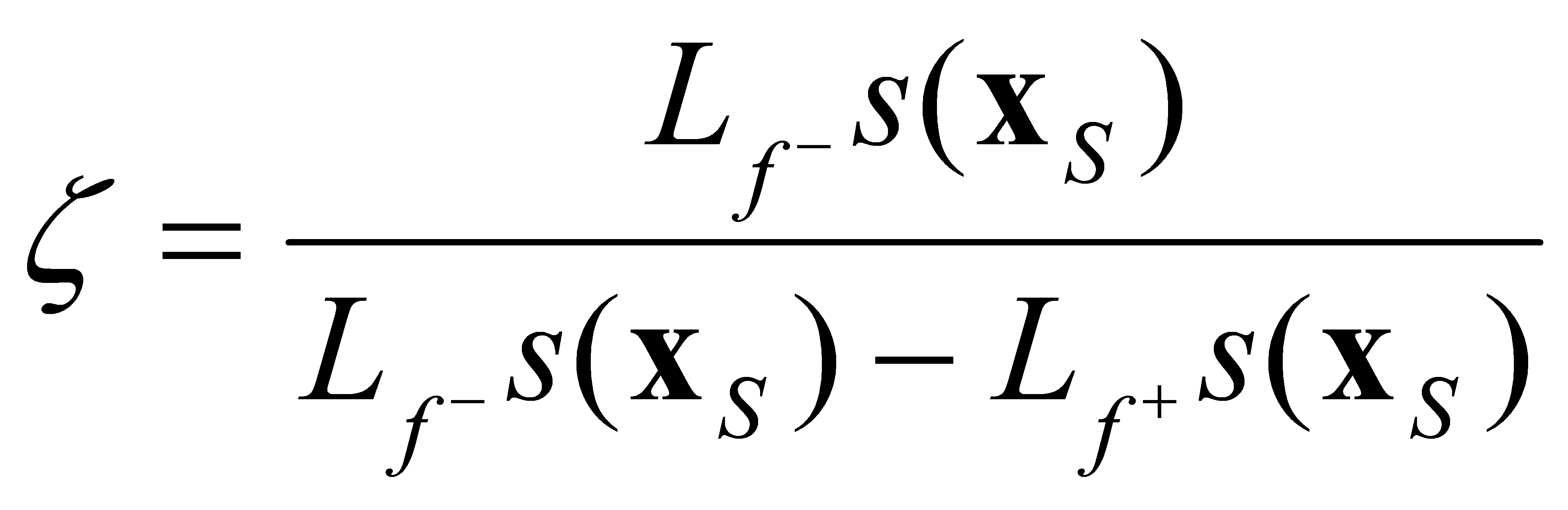
From (4.23) can be expressed:

(4.24)

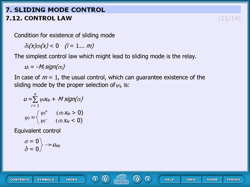
4.4.1. Condition for the existence of Sliding Mode

If $L_{f^{+}} s (x_{S}) < 0$ and $L_{f^{-}} s (x_{S}) > 0$ then on both sides of the surface S the vector space f(x) points towards the surface S (see Figure 4-6.). Therefore, if the state trajectory once reaches the surface S, it can not leave it. The state trajectory slides along the surface and therefore this state is called sliding mode.

Figure 4.6. The f(x) vector space pointing towards the surface S.

Note that the two conditions separately defined on both sides of the surface S:

$L_{f^{+}} s (x) < 0, if x \in Q (x_{S}, δ) \cap G^{+}$	(4.25)
$L_{f^{-}} s (x) > 0, if x \in Q (x_{S}, δ) \cap G^{-}$	(4.26)

can be substituted by one inequality:

$\frac{d}{d t} s {(x)}^{2} < 0, if x \in Q (x_{S}, δ) - S$

(4.27)

Which can be interpreted as Lyapunov's stability criterion concerning whether the system remains on the surface S.

4.5. The solution of the differential equation of the introductory example

There are two energy storage elements (L and C) in the circuit of the introductory example, therefore the behavior of the circuit can be described by two state variables. The goal is to remove the voltage error, so it is practical to choose the error signal and the first time derivative of it as the state variables.

$x = [\begin{matrix} u_{e} \\ \frac{d}{d t} u_{e} \end{matrix}] = [\begin{matrix} U_{r} - u_{c} \\ - \frac{d}{d t} u_{c} \end{matrix}]$

(4.28)

The state equation of the error signal, assuming that the reference signal Ur is constant:

$\frac{d}{d t} [\begin{matrix} u_{e} \\ \frac{d}{d t} u_{e} \end{matrix}] = [\begin{matrix} 0 & 1 \\ - \frac{1}{L C} & a_{22} \end{matrix}] [\begin{matrix} u_{e} \\ \frac{d}{d t} u_{e} \end{matrix}] + [\begin{matrix} 0 \\ \frac{1}{L C} \end{matrix}] (U_{r} - u_{A B})$

(4.29)

where a22 = 0, if we neglect the losses assuming ideal L-C elements, while a22 = -R/L, if we model the losses of the circuit with serial resistance. Based on (4.6) and (4.7), let the scalar function defining, the sliding surface be:

$s (x) = [1 λ] [\begin{matrix} u_{e} \\ \frac{d}{d t} u_{e} \end{matrix}]$

(4.30)

Rewriting the matrix equation (4.29) to the form (4.17), we obtain:

$\frac{d}{d t} x = f (x) = {\begin{matrix} f^{+} (x) = [\begin{matrix} f_{1} \\ f_{2} - u_{+} \end{matrix}], if the switch is in state 1 \\ f^{-} (x) = [\begin{matrix} f_{1} \\ f_{2} \end{matrix}], if the switch is in state 2 \end{matrix}$

(4.31)

where

$f_{1} = \frac{d}{d t} u_{e}$	(4.32)
$f_{2} = - \frac{1}{L C} u_{e} - a_{22} \frac{d}{d t} u_{e} + \frac{1}{L C} U_{r}$	(4.33)
$u_{+} = \frac{1}{L C} U_{b a t}$	(4.34)

The directional derivative of the scalar function s(x) concerning the vector space f(x) on both sides of the surface S is:

$L_{f^{+}} s (x_{s}) = \frac{d}{d t} u_{e s} + λ (- \frac{1}{L C} u_{e s} - a_{22} \frac{d}{d t} u_{e s} - u_{+}) = f_{1 s} + λ (f_{2 s} - u_{+})$	(4.35)
$L_{f^{-}} s (x_{s}) = \frac{d}{d t} u_{e s} + λ (- \frac{1}{L C} u_{e s} - a_{22} \frac{d}{d t} u_{e s}) = f_{1 s} + λ f_{2 s}$	(4.36)

Note that in our case f +(x) and f -(x) can be defined on the surface S, therefore we do not need to calculate the limits in (4.21), the points $u_{e s}, \frac{d}{d t} u_{e s}$ belonging to the surface S can be directly substituted. At the same time, (4.27) is met only in the following domain:

(4.37)

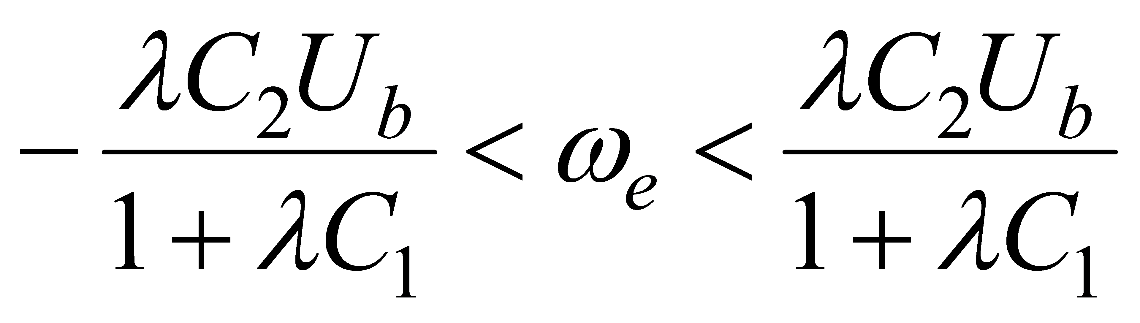
It means that, by the given control relay, only on a limited part of the surface S can be in sliding mode. By completing the relay control laws with additional members, we can reach that the condition of sliding mode is fulfilled on the whole S surface [5] [6]. In case of the control relay, based on (4.24) and (4.35), we get:

(4.38)

Based on (4.17), (4.31), (4.35), and (4.38) the differential equation describing the system in sliding mode will be:

$\frac{d}{d t} [\begin{matrix} u_{e s} \\ \frac{d}{d t} u_{e s} \end{matrix}] = \frac{f_{1 s} + λ f_{2 s}}{λ u_{+}} [\begin{matrix} f_{1 s} \\ f_{2 s} - u_{+} \end{matrix}] + \frac{λ u_{+} - f_{1 s} - λ f_{2 s}}{λ u_{+}} [\begin{matrix} f_{1 s} \\ f_{2 s} \end{matrix}] = [\begin{matrix} f_{1 s} \\ - \frac{1}{λ} f_{1 s} \end{matrix}]$

(4.39)

The differential equation (4.39) is basically the same as the equation of the sliding line, and thus we can describe the original system as a first order differential equation instead of a second order one:

$s (x_{s}) = 0 = u_{e s} + λ \frac{d}{d t} u_{e s}$

(4.40)

This way we proved, that the state belonging to the smooth regular sliding line S can be accurately followed by a state trajectory broken in each points consisting of infinitely short sections switched by infinitely high frequency. The solution of (4.40) is:

$u_{e s} = U_{e s 0} e^{- \frac{1}{λ} t}$

(4.41)

where Ues0 is the ues error signal at the moment when the state trajectory reaches the surface S. Based on (4.41) we can see that $λ$ is the characteristic time constant of the sliding line. Note that equation (4.41) does not include any parameter of the original system. This means that in the above-described ideal sliding mode the relay control law leads to a robust controller, insensitive to certain parameters and disturbances. The above derivation is only concerned with how the system behaves on the sliding surface, but we did not deal with the practically very important question of how to ensure that the state trajectory always reaches the sliding surface and stays on it.

Of course, in reality such an ideal sliding mode does not exist. From engineering point of view the challenge is the realization of a so-called chattering-free approximation of it.

4.6. Design of the sliding manifold is state-space approach

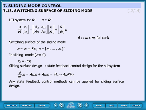
The following linear time invariant (LTI) system is considered; first the reference signal is supposed to be constant and zero.

$\dot{x} = A x + B u$ , $x \in R^{n}, u \in R^{m}$

(4.42)

$y = C x + D u$ $y \in R^{l}, l \leq n$

(4.43)

The system (4.42) can be transformed to a regular form:

$[\begin{matrix} {\dot{x}}_{1} \\ {\dot{x}}_{2} \end{matrix}] = [\begin{matrix} A_{11} & A_{12} \\ A_{21} & A_{22} \end{matrix}] \cdot [\begin{matrix} x_{1} \\ x_{2} \end{matrix}] + [\begin{matrix} 0 \\ B_{2} \end{matrix}] \cdot u$

(4.44)

where $x_{1} \in R^{n - m}, x_{2} \in R^{m}$

The switching surfaces of the sliding mode, where the control vector components have discontinuities, can be written in the following form:

$σ = x_{2} + K x_{1}$ $σ \in R^{m}$

(4.45)

When sliding mode occurs, σ = x2 + Kx1 and x2 = -Kx1. The design problem of the sliding surfaces can be regarded as a linear state feedback control design for the following subsystem:

${\dot{x}}_{1} = A_{11} x_{1} + A_{12} x_{2}$

(4.46)

In (4.46) equation, x2 can be considered as the input of the subsystem. A state feedback controller x2 = = -Kx1 for this subsystem gives the switching surface of the whole VSS controller. In sliding mode

${\dot{x}}_{1} = (A_{11} - A_{12} K) x_{1}$

(4.47)

Various linear control design methods based on state feedback are applicable to the design of the switching surfaces.

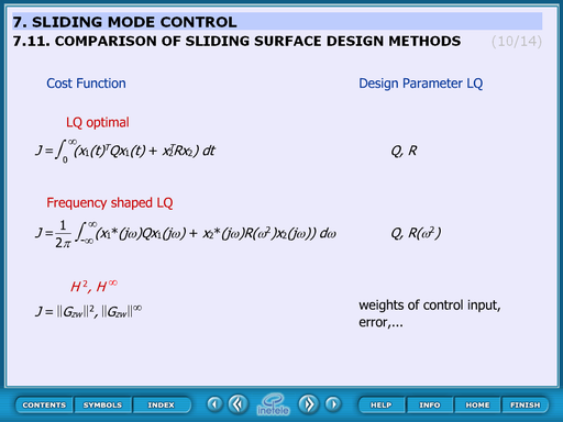
4.6.1. Linear Quadratic approach

According to LQ design the cost function (4.48) is minimized by solving the well known Riccati equation to achieve the optimal feedback gain for subsystem (4.46):

$J = \int_{t_{s}}^{\infty} (x_{1}^{T} Q x_{1} + 2 x_{1}^{T} N x_{2} + x_{2}^{T} R x_{2}) d t .$

(4.48)

where ts (can be assumed zero) is the time at which sliding mode begins. (For simplicity, N = 0 is assumed.)

The LQ optimal sliding surface is given by

$K_{L Q} = R^{- 1} A_{12}^{T} P$ , $σ = x_{2} + K_{L Q} x_{1}$

(4.49)

where P > 0 is a unique solution of the following Riccati equation:

$P A_{11} + A_{11}^{T} P - P A_{12} R^{- 1} A_{12}^{T} P + Q = 0$

(4.50)

4.6.2. Frequency shaped LQ approach

The frequency shaped sliding mode comes from frequency shaped LQ method. Frequency shaped LQ approach is based on frequency dependent weights. The cost function (4.48) can be written in the frequency domain using Perseval's theorem as

$J = \frac{1}{2 π} \int_{- \infty}^{\infty} (x_{1}^{T} (j ω) Q x_{1} (j ω) + x_{2}^{T} (j ω) R x_{2} (j ω)) d ω .$

(4.51)

In the time domain (4.48), Q and R are constant matrices. If instead of a constant R, a frequency dependent weight matrix R(ω2) is introduced, control inputs for certain frequencies can be amplified or suppressed.

$J = \frac{1}{2 π} \int_{- \infty}^{\infty} (x_{1}^{T} (j ω) Q x_{1} (j ω) + x_{2}^{T} (j ω) R (ω^{2}) x_{2} (j ω)) d ω .$

(4.52)

We can choose R to have high-pass characteristics for reduction of high frequency control inputs of the subsystem (4.46).

This idea is realized using state space representation. The frequency dependent weight R(ω2) must be a rational function of ω2 to solve this problem. The transfer function matrix W2(s) is defined as

$R (ω^{2}) = W_{2} (j ω) * W_{2} (j ω)$

(4.53)

where W2(s)* stands for the conjugate transpose of W2(s). The subsystem (4.46) should be augmented by the states (written in the vector xw2) of W2(s). W2(s) has the following state space representation

$\begin{array}{l} \tilde{u} = W_{2} (s) x_{2} \\ \frac{d}{d t} x_{w 2} = A_{w 2} x_{w 2} + B_{w 2} x_{2} \\ \tilde{u} = C_{w 2} x_{w 2} + D_{w 2} x_{2} \end{array}$

(4.54)

Then the cost function (4.52) with a frequency dependent weight matrix R(ω2) can be rewritten in the time domain as

$J = \int_{0}^{\infty} (x_{a}^{T} Q_{a} x_{a} + 2 x_{a}^{T} N_{a} x_{2} + x_{2}^{T} R_{a} x_{2}) d t .$

(4.55)

where

${\dot{x}}_{a} = A_{a} x_{a} + B_{a} x_{2}, x_{a} = [\begin{matrix} x_{w 2} \\ x_{1} \end{matrix}],$	(4.56)
$\begin{array}{l} A_{a} = d i a g (A_{w 2}, A_{11}), B_{a} = [\begin{matrix} B_{w 2} \\ A_{12} \end{matrix}], \\ Q_{a} = d i a g (C_{w 2}^{T} C_{w 2}, Q), N_{a} = [\begin{matrix} C_{w 2}^{T} D_{w 2} \\ 0 \end{matrix}], \\ R_{a} = D_{w 2}^{T} D_{w 2} . \end{array}$	(4.57)

Minimization of this cost function with cross term between state and control input is formulated as solving the following Riccati equation:

$P_{a} A_{a} + A_{a}^{T} P_{a} - (P_{a} B_{a} + N_{a}) R_{a}^{- 1} (B_{a}^{T} P_{a} + N_{a}^{T}) + Q_{a}^{T} = 0$

(4.58)

The optimal switching plane is written using the solution of this Riccati equation as

$K_{F S} = R_{a}^{- 1} (B_{a}^{T} P_{a} + N_{a}^{T}) .$ $σ = x_{2} + K_{F S} x_{a}$

(4.59)

4.6.3. H∞ optimal control approach

Recently, linear control theory is well developed especially in the field of robust control. H∞ optimal control theory is an excellent result of this development. Hashimoto introduces H∞ control methods for the optimal sliding surface design based on H∞ norm.

The control goal is formulated through a norm minimization of the generalized plant G(jω), where H∞ norms are used to formulate the cost function. If G(jω) is a stable transfer matrix in the frequency domain, than the H∞ norms are

${‖ G (s) ‖}^{\infty} = \sup_{ω} σ_{\max} [G (j ω)] .$

(4.60)

4.7. Discrete-time sliding mode design

Another kind of chattering is caused by the limited switching frequency of the control input. The robustness of continuous-time sliding mode control is obtained by high frequency switching of high-gain control inputs. To adapt the sliding-mode philosophy for a digital controller, the sampling frequency should be increased compared to other types of control method. To solve this problem asymptotic reaching of the sliding manifold has been proposed in literatures to avoid commutation. In an alternative idea, the samples of the system states belong to the sliding manifold after a finite number of sample steps.

Definition:

In the discrete-time dynamic system

$S_{i} : = {x : s_{i} (x) = 0} i = 1, 2 \dots m .$	(4.61)
$x_{k + 1} = F (x_{k})$ $x \in ℜ^{n}$	(4.62)

a discrete-time sliding mode takes place on the subset of a manifold $s (x) = 0, s \in ℜ^{m} (m < n)$ if there exists an open neighborhood U of this subset such that from $x \in U$ it follows $s (F (x)) \in Σ$ .

According to this definition, the observer equation should be discretized at each sampling instant.

${\hat{x}}_{k + 1} = A_{d} {\hat{x}}_{k} + B_{d} u_{k}$

$\dot{x} = A x + B u \to$

(4.63)

where subscript k means the k-th sampling time, i.e., t = kTs (Ts is the sampling period) and

$A_{d} = e^{A T_{s}},$ $B_{d} = \int_{0}^{T_{s}} e^{A (T_{s} - τ)} B d τ$

(4.64)

The sliding surface should be discretized as well:

$σ_{k} = Λ_{d} x_{e k}$ , $σ = Λ x_{e} = 0 \to$

(4.65)

It follows from the definition that

$σ_{k + 1} = 0$

(4.66)

for any $x_{k} \in U$ . The discrete-time sliding mode exists if matrix $Λ_{d} B_{d}$ is invertible and control Uk is designed to satisfy (4.46):

$σ_{k + 1} = Λ_{d} x_{e k + 1} = Λ_{d} (x_{r k + 1} - A_{d} x_{k} - B_{d} u_{k})$

(4.67)

By analogy with continuous-time systems, the solution of (4.67) is referred to as “equivalent control”.

$u_{e q k} = {(Λ_{d} B_{d})}^{- 1} Λ_{d} (x_{r k + 1} - A_{d} x_{k})$

(4.68)

The control law is chosen as follows:

$u_{k} = {\begin{cases} u_{e q k} \\ u_{\max} \frac{u_{e q k}}{‖ u_{e q k} ‖} \end{cases}$ $\begin{matrix} (‖ u_{e q k} ‖ < u_{\max}) \\ (‖ u_{e q k} ‖ > u_{\max}) \end{matrix}$

(4.69)

where $U_{\max}$ is the physical limit of control signal $u_{k}$ .

This type of discrete-time sliding mode control law involves prediction. Knowledge of the model is necessary.

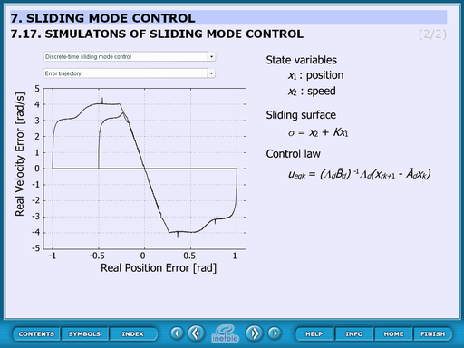
4.8. Sliding mode Introductory example

Figure 4.7. Introductory example

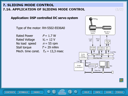
This static slide contains the basic idea of the sliding mode control. The controller plant is a DC motor, the actuator is a DC-DC converter and the control method is bang-bang.

This means that the DC motor is controller by a 2 state kind of relay which can accelerate or decelerate the motor. This control can switch when the system approaches the reference position but this causes big overshoot therefore the switching process must be occurred a little bit before that time. The question is: when. The next some slides give us the answer.

4.8.1. Derivation of system trajectory

Figure 4.8. System trajectory

The bases of the transfer function are these equations:

$V_{a} = i_{a} R_{a} + L_{a} \frac{d i_{a}}{d t} + k φ Ω$

(4.70)

$T_{E} = k \cdot φ \cdot i_{a}$

(4.71)

$T_{E} - T_{L} = J \frac{d Ω}{d t}$

(4.72)

And the transfer function:

Figure 4.9. System trajectory

The basic of this derivation is the transfer function:

$V_{a} = \frac{L_{a} J}{k φ} \frac{d^{2} Ω}{d t^{2}} + k φ Ω + \frac{R_{a} J}{k φ} \frac{d Ω}{d t} + \frac{R_{a}}{k φ} T_{L} + \frac{L_{a}}{k φ} \frac{d T_{L}}{d t}$

(4.73)

where the 3rd, 4th and the 5th member can be neglected (red cross shows the neglecting):

$\frac{R_{a} J}{k φ} \frac{d Ω}{d t} + \frac{R_{a}}{k φ} T_{L} + \frac{L_{a}}{k φ} \frac{d T_{L}}{d t}$

(4.74)

herefore:

$V_{a} = \frac{L_{a} J}{k φ} \frac{d^{2} Ω}{d t^{2}} + k φ Ω$

(4.75)

Introducing the “per unit”:

$τ = \frac{k φ}{\sqrt{J L_{a}}}$

(4.76)

The non-load speed:

$ω_{n l} = \ddot{ω} + ω$

(4.77)

Figure 4.10. Error trajectory

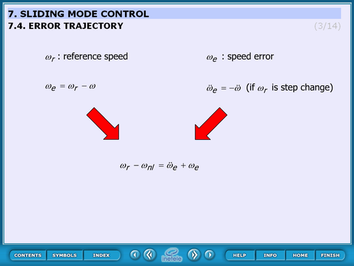
This slide derives the error trajectory.

$ω_{r}$ – reference speed

$ω_{e} = ω_{r} - ω$

(4.78)

$ω_{e}$ – speed error

${\ddot{ω}}_{e} = - \ddot{ω}$

(4.79)

if $ω_{r}$ is the step change

$ω_{r} - ω_{n l} = {\ddot{ω}}_{e} + ω_{e}$

(4.80)

4.8.2. Error trajectory

Figure 4.11. Error trajectory

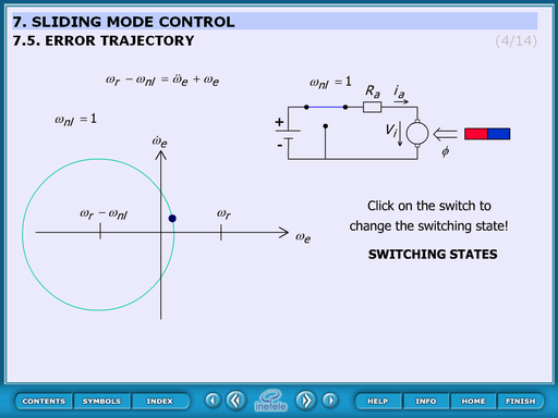
This animated figure displays the error trajectory when the switch is on or off.

Theoretical background:

The motor can be considered as a second order storage element which responds to the step change with oscillation. This oscillation appears as a circle in the ( $ω_{e}$ ; ${\dot{ω}}_{e}$ ) diagram. The centre of the circle is $ω_{r} - ω_{n l}$ when the switch is on ( $ω_{n l} = 1$ ) and $ω_{r}$ when the switch is off ( $ω_{n l} = 0$ ).

Operation:

At start-up the switch is on and by clicking the switch it can be toggled between on and off state.

4.8.3. Simple switching strategy

Figure 4.12. Simple switching strategy

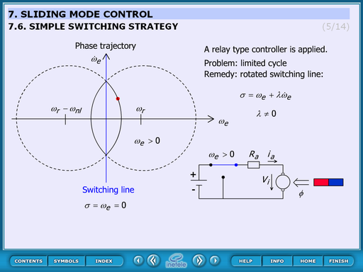
This animation sows the problem in case of the simplest control strategy. The process: the controller accelerates the motor until it reaches the reference speed. At this moment it switches and decelerates. But the system stores a lot of energy therefore overshoots. At the end of the overshoot the speed is higher than the reference and the system starts really slowing. But reaching again the reference speed and switching on the system would not accelerate immediately because of the storage capability. This process repeats and oscillation occurs.

$σ = ω_{e} + λ {\dot{ω}}_{e}$	(4.81)
$λ \neq 0$	(4.82)
$σ = ω = 0$	(4.83)

The switching line is horizontal. To solve the oscillation problem the switching line should be rotated.

The animation cannot be controller actually. In the future built in buttons can be implemented is required.

4.8.4. Explanation of sliding mode

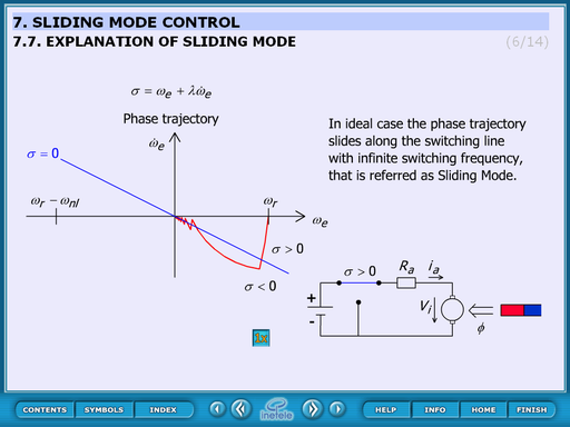
Figure 4.13. Explanational animated figure about sliding mode control

This animated figure explains the effect of the rotated switching line.

The trajectory slides from $ω_{r}$ in the direction of the switching line. When reaches the centre of the circle changes and the curve again to the direction of the sw. line.

The control of the animation:

It starts automatically and at the end it can be restarted by pressing button.

This animation uses previously drawn figure. There is the possibility of changing this to function.

4.8.5. Robustness of sliding mode control

Figure 4.14. Robustness

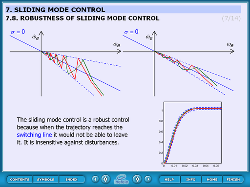
This static figure explains the robustness of the sliding mode control.

Theoretical background:

Once the control reaches the switching line the system becomes insensitive against disturbances because it won’t be able to leave the line. The way in which it reaches the line is independent from the result.

4.8.6. Time function

Figure 4.15. Time function

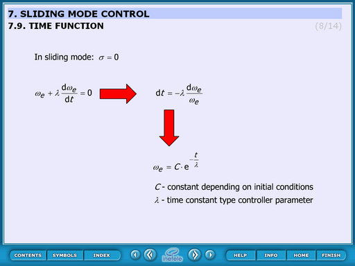
This animated slide derives the time function. Equations:

In sliding mode:

$σ = 0$

(4.84)

$ω_{e} + λ \frac{d ω_{e}}{d t} = 0$

(4.85)

$d t = - λ \frac{d ω_{e}}{ω_{e}}$

(4.86)

$ω_{e} = C \cdot e^{- \frac{t}{λ}}$

(4.87)

Where:

C – constant depends on initial conditions

- time constant type controller parameter

4.8.7. Design of Sliding mode control

Figure 4.16. Design of Sliding mode control

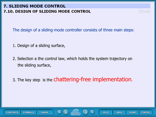
This slide concludes the screens until now. The text of the slide:

The design of a sliding-mode controller consists of three main steps:1. Design of a sliding surface, 2. Selection a the control law, which holds the system trajectory on the sliding surface,3. The key step is the chattering-free implementation.