Chapter 3. Environment Sensing (Perception) Layer
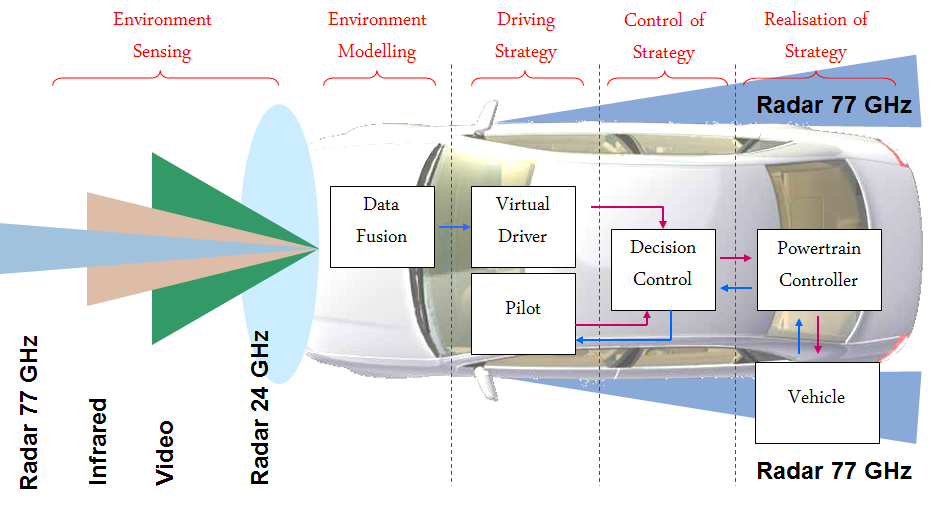
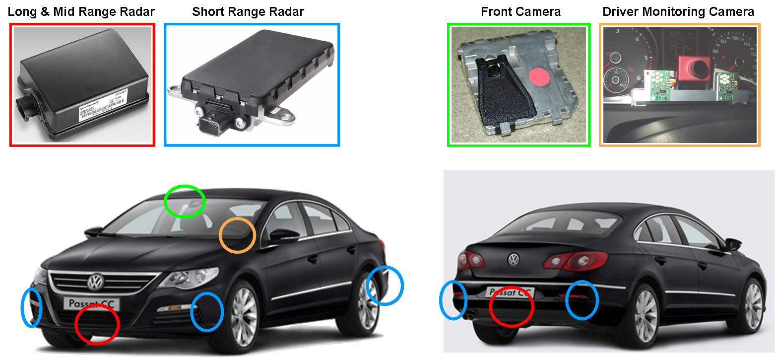
The task of the environment sensing layer is to provide comprehensive information about the surrounding objects around the vehicle. There are different types of sensors installed all around the vehicle that deliver information from near, medium and distant ranges. The following figure shows the elements of the environment sensing around the vehicle.
The vehicle sensor devices can be classified according to the aforementioned viewpoints:
-
Near distance range
-
Radar (24GHz)
-
Video
-
3D Camera
-
Medium distance range
-
Video
-
Far distance range
-
Radar (77/79GHz)
-
Lidar
3.1. Radar
Automotive radar sensors are responsible for the detection of objects around the vehicle and the detection of hazardous situations (potential collisions). A positive detection can be used to warn/alert the driver or in higher level of vehicle automation to intervene with the braking and other controls of the vehicle in order to prevent an accident. The basic theory of radar systems is explained in the following chapters based on [29].
In an automotive radar system, one or more radar sensors detect obstacles around the vehicle and their speeds relative to the vehicle. Based on the detection signals generated by the sensors, a processing unit determines the appropriate action needed to avoid the collision or to reduce the damage (collision mitigation).
Originally the word radar is an acronym for RAdio Detection And Ranging. The measurement method is the active scanning i.e. the radar transmits radio signal and the reflected signal is analysed. The main advantages of the radar are the lower costs and the weather-independency.
The basic output information of the automotive radars is the followings:
-
Detection of objects
-
Relative position of the objects to the vehicle
-
Relative speed of the objects to the vehicle
Based on this information the following user-level functionalities can be implemented:
-
Alert the driver about any potential danger
-
Prevent collision by intervening with the control of the vehicle in hazardous situations
-
Take over partial control of the vehicle (e.g., adaptive cruise control)
-
Assist the driver in parking the car
Radar operation can be divided into two major tasks:
-
Distance detection
-
Relative speed detection
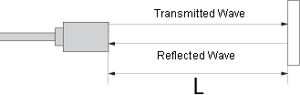
Distance detection can be performed by measuring the round-trip duration of a radio signal. Based on the wave speed in the medium, it will take a certain time for the transmitted signal to travel, be reflected from the target, and travel back to the radar receiver. By measuring this time interval that the signal has travelled the distance can easily be calculated.
The underlying concept in the theory of speed detection is the Doppler frequency shift. A reflected wave from a moving object will experience a frequency change, depending on the relative speed and direction of movement of the source that has transmitted the wave and the object that has reflected the wave. If the difference between the transmitted signal frequency and received signal frequency can be measured, the relative speed can also be calculated.
According to the type of transmission the radar system can be continuous wave (CW) or pulsed. In continuous-wave (CW) radars, a high-frequency signal is transmitted and by measuring the frequency difference between the transmitted and the received signal (Doppler frequency), the speed of the reflector object can be quite well estimated.
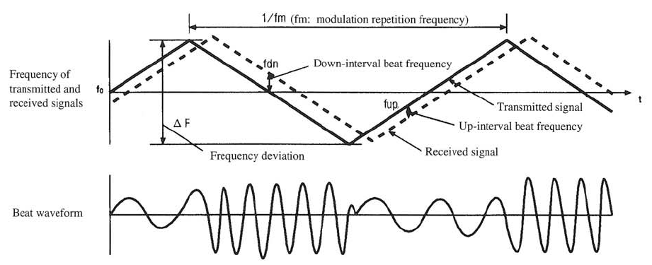
The most widely used technology is the FM-CW (Frequency Modulated Continuous Wave). In FMCW radars, a ramp waveform or a saw-tooth waveform is used to generate a signal with linearly varying frequency in time domain. The high-frequency transmitted signal emitted from the sensor is modulated using a frequency f0, modulation repetition frequency is fm, and frequency deviation is ΔF. The radar signal is reflected by the target, and the radar sensor receives the reflected signal. Beat signals (see Figure 32 [30]) are obtained from the transmitted and received signals and the beat frequency is proportional to the distance between the target and the radar sensor. Relative speed and relative distance can be determined by measuring the beat frequencies.
In pulsed radar architectures, a number of pulses are transmitted and from the time delay and change of pulse width that the transmitted pulses will experience in the round trip, the distance and the relative speed of the target object can be estimated. Transmitting a narrow pulse in the time domain means that a large amount of power must be transmitted in a short period of time. In order to avoid this issue, spread spectrum techniques may be used.
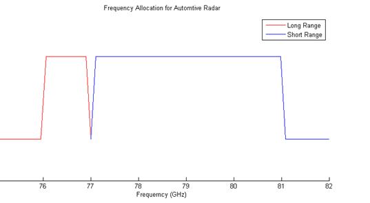
There are 4 major frequency bands allocated for radar applications, which can be divided into two sub-categories: 24-GHz band and 77-GHz band.
The 24-GHz band consists of two sub-bands, one around 24.125GHz with a bandwidth of around 200MHz and, the other around 24GHz with a bandwidth of 5GHz. Both of these bands can be used for short/mid-range radars.
The 77-GHz band also consists of two sub-bands, 76-77GHz for narrow-band long-range radar and 77-81GHz for short-range wideband radar (see Figure 33 [29]).
As frequency increases, smaller antenna size can be utilized. As a result, by going toward higher frequencies angular resolution can be enhanced. Furthermore, by increasing the carrier frequency the Doppler frequency also increases proportional to the velocity of the target; hence by using mm-wave frequencies, a higher speed resolution can be achieved. Range resolution depends on the modulated signal bandwidth, thus wideband radars can achieve a higher range resolution, which is required in short-range radar applications. Recently, legal authorities are pushing for migration to mm-wave range by imposing restrictions on manufacturing and power emission in the 24GHz band. It is expected that 24-GHz radar systems will be phased out in the next few years (at least in the EU countries). This move will help eliminate the issue of the lack of a worldwide frequency allocation for automotive radars, and enable the technology to become available in large volumes.
By using the 77-GHz band for long-range and short-range applications, the same semiconductor technology solutions may be used in the implementation of both of them. Also, higher output power is allowed in this band, as compared to the 24-GHz radar band. 76-77-GHz and 77-81-GHz radar sensors together are capable of satisfying the requirements of automotive radar systems including short-range and long-range object detection. For short-range radar applications, the resolution should be high; as a result, a wide bandwidth is required. Therefore, the 77-81-GHz band is allocated for short-range radar (30-50m). For long-range adaptive cruise control, a lower resolution is sufficient; as a result, a narrower bandwidth can be used. The 76-77-GHz is allocated for this application.
As an explanation of the above mentioned range classification, the automotive radar systems can be divided into three sub-categories: short-range, mid-range and long-range automotive radars. For short-range radars, the main aspect is the range accuracy, while for mid-range and long-range radar systems the key performance parameter is the detection range.
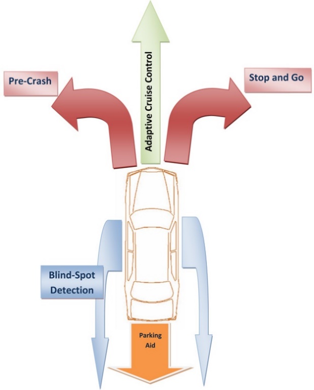
Short-range and mid-range radar systems (range of tens of meters) enable several applications such as blind-spot detection and pre-crash alerts. It can also be used for implementation of “stop–and-go” traffic jam assistant applications in city traffic.
Long-range radars (hundreds of meter) are utilized in adaptive cruise-control systems. These systems can provide enough accuracy and resolution for even relatively high speeds.
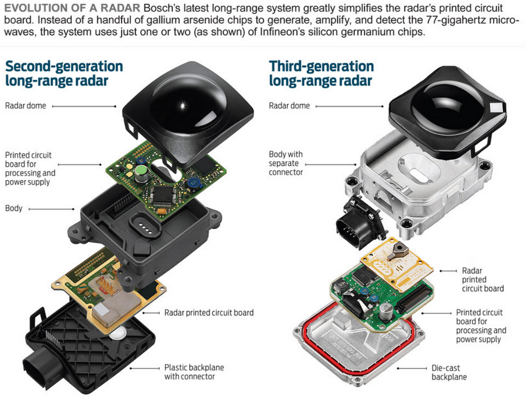
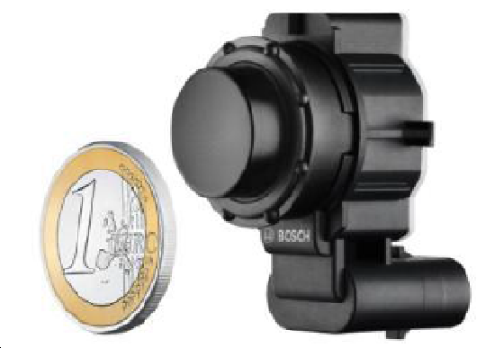
Nowadays the most significant OEMs can integrate the radar functionality into a small and relatively low cost device. When Bosch upgraded Infineon's product during the development of its third-generation long-range radar (dubbed, unimaginatively, the LRR3), both the minimum and maximum ranges of its system got better: The minimum range dropped from 2 meters to half a meter, and the maximum range shot from 150 to 250 meters. At the same time, the detection angle doubled to 30 degrees, and the accuracy of angle and distance measurements increased fourfold. The superiority originates from the significantly higher radar bandwidth used in the systems containing the silicon-based chips. Another point is the new system's compact size—just 7.4 by 7 by 5.8 centimetres.
The system utilizes four antennas and a big plastic lens to shoot microwaves forward and also detect the echoes, meanwhile ramping the emission frequency back and forth over 500-MHz band. (Because the ramping is so fast, the chance of two or more radars interfering is extraordinarily low.) The system compares the amplitudes and phases of the echoes, pinpointing each car within range to within 10 cm in distance and 0.1 degree in displacement from the axis of motion. Then it works out which cars are getting closer or farther away by using the Doppler Effect. In all, the radar can track 33 objects at a time. (Source[31])
The following table shows the main properties of the Continental’s ARS300 Long- and Mid-range Rader.
|
Range (Measured using corner reflector, 10 m² RCS) |
0.25m up to 200m far range scan 0.25m up to 60m medium range scan |
|
Field of view |
field of view conform with the ISO classes I ... IV azimuth 18° far range scan 56° medium range scan elevation 4.3° (6dB beam width) |
|
Cycle time |
66 ms (far and medium range scan in one cycle) |
|
Accuracy |
range 0.25m, no ambiguities angle 0.1° complete far distance field of view 1.0° medium range (0° < || < 15°) 2.0° medium range (15° < || < 25°) speed (-88 km/h ... +265 km/h; extended to all realistic velocities by tracking software) 0.5 km/h |
|
Resolution |
range 0.25m (d < 50m) 0.5m (50m < d < 100m) 1m (100m < d < 200m) |
3.2. Ultrasonic
Ultrasonic sensors are industrial control devices that use sound waves above 20 000 Hz, beyond the range of human hearing, to measure and calculate distance from the sensor to a specified target object. This sensor technology is detailed here from [32].
The sensor has a ceramic transducer that vibrates when electrical energy is applied to it. This phenomenon is called piezoelectric effect. The word piezo is Greek for "push". The effect known as piezoelectricity was discovered by brothers Pierre and Jacques Curie when they were 21 and 24 years old in 1880. Crystals which acquire a charge when compressed, twisted or distorted are said to be piezoelectric. This provides a convenient transducer effect between electrical and mechanical oscillations. Quartz demonstrates this property and is extremely stable. Quartz crystals are used for watch crystals and for precise frequency reference crystals for radio transmitters. Rochelle salt produces (Potassium sodium tartrate) a comparatively large voltage upon compression and was used in early crystal microphones. Several ceramic materials are available which exhibit piezoelectricity and are used in ultrasonic transducers as well as microphones. If an electrical oscillation is applied to such ceramic wafers, they will respond with mechanical vibrations which provide the ultrasonic sound source.
The vibrations compress and expand air molecules in waves from the sensor face to a target object. A transducer both transmits and receives sound. The ultrasonic sensor will measure distance by emitting a sound wave and then listening for a set period of time, allowing for the return echo of the sound wave bouncing off the target before retransmitting (pulse-echo operation mode).
The sensor emits a packet of sonic pulses and converts the echo pulse into a voltage. The controller computes the distance from echo time and the velocity of sound. The velocity of sound in the atmosphere reaches 331.45 m/s when the temperature is 0°C. The sound velocity at different temperatures can be calculated with the following formula. Sound velocity increases by 0.607 m/s every time the temperature rises 1°C.
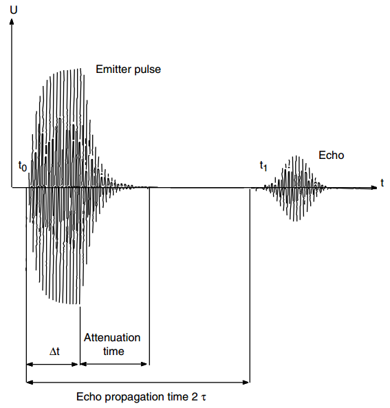
The emitted pulse duration Δt and the attenuation time of the sensor result in an unusable area in which the ultrasonic sensor cannot detect and object. That is why the limited minimum detection range is around 20 cm.
Ultrasonic sensors use sound rather than light for detection, they work in applications where photoelectric sensors may not. Ultrasonic sensors are a great solution for clear object detection and for liquid level measurement, applications that photoelectric struggle with because of target translucence. Target colour and/or reflectivity don't affect ultrasonic sensors which can operate reliably in high-glare environments. Ultrasonic sensors definitely have advantages when sensing clear objects, liquid level or highly reflective or metallic surfaces. Ultrasonic sensors also function well in wet environments where as an optical beam may refract off the water droplets. On the other hand ultrasonic sensors are susceptible to temperature fluctuations or wind.
In the automotive industry the ultrasonic sensors are mainly used for parking aid and blind-spot functions. These sensors typically work at ~48 kHz operating frequency with a detection range of 25-400 cm. The opening angle is about 120° horizontally and 60° vertically.
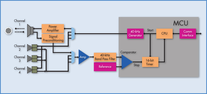
The general architecture of automotive ultrasonic systems is shown on Figure 38. It consists of the ultrasonic sensors mounted into the front and rear bumpers, the analogue amplifiers and filters and the ECU. The main unit of the ECU (generally a microcontroller) generates the signal and drives the sensors by the power amplifier. The generated sound wave reflects off an object and is converted back to electronic signal with the same sensor element. The MCU measures the echo signal, evaluates and calculates the distances. Generally the results are broadcasted by high-level communication interface such as CAN, or sent directly to an HMI for further processing.
3.3. Video camera
The recording capabilities of the automotive video cameras are based on image sensors (imagers). It is the common name of those digital sensors which can convert an optical image into electronic signals. Currently used imager types are semiconductor based charge-coupled devices (CCD) or active pixel sensors formed of complementary metal–oxide–semiconductor (CMOS) devices. These main image capture technologies are introduced based on the comparison in [33].
Both image sensors are pixelated semiconductor structures. They accumulate signal charge in each pixel proportional to the local illumination intensity, serving a spatial sampling function. When exposure is complete, a CCD (Figure 39 [33]) transfers each pixel’s charge packet sequentially to a common output structure, which converts the charge to a voltage, buffers it and sends it off-chip. In a CMOS imager (Figure 40 [33]), the charge-to-voltage conversion takes place in each pixel. This difference in readout techniques has significant implications for sensor architecture, capabilities and limitations.
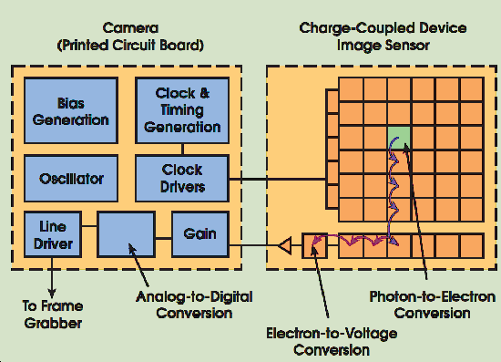
On a CCD, most functions take place on the camera’s printed circuit board. If the application demands hardware modifications, a designer can simply change the electronics without redesigning the imager.
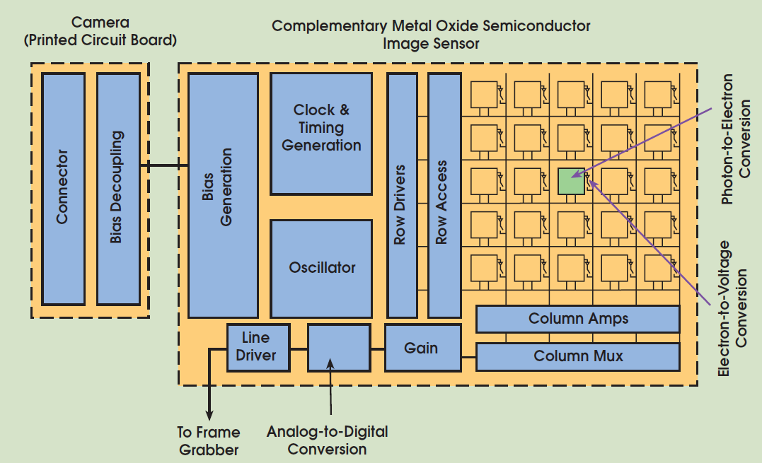
A CMOS imager converts charge to voltage at the pixel, and most functions are integrated into the chip itself. This makes imager functions less flexible but, for applications in rugged environments, a CMOS camera can be more reliable.
3.3.1. Image sensor attributes
As defined in [33] there are eight attributes that characterize image sensor performance. This attributes will be explained in details in the following paragraphs:
Responsivity, the amount of signal the sensor delivers per unit of input optical energy. CMOS imagers are marginally superior to CCDs, in general, because gain elements are easier to place on a CMOS image sensor. Their complementary transistors allow low-power high-gain amplifiers, whereas CCD amplification usually comes at a significant power penalty. Some CCD manufacturers are challenging this concept with new readout amplifier techniques.
Dynamic range, the ratio of a pixel’s saturation level to its signal threshold. It gives CCDs an advantage by about a factor of two in comparable circumstances. CCDs still enjoy significant noise advantages over CMOS imagers because of quieter sensor substrates (less on-chip circuitry), inherent tolerance to bus capacitance variations and common output amplifiers with transistor geometries that can be easily adapted for minimal noise. Externally coddling the image sensor through cooling, better optics, more resolution or adapted off-chip electronics cannot make CMOS sensors equivalent to CCDs in this regard.
Uniformity, the consistency of response for different pixels under identical illumination conditions. Ideally, behaviour would be uniform, but spatial wafer processing variations, particulate defects and amplifier variations create non-uniformities. It is important to make a distinction between uniformity under illumination and uniformity at or near dark. CMOS imagers were traditionally much worse under both regimes. Each pixel had an open-loop output amplifier, and the offset and gain of each amplifier varied considerably because of wafer processing variations, making both dark and illuminated non-uniformities worse than those in CCDs. Some people predicted that this would defeat CMOS imagers as device geometries shrank and variances increased. However, feedback-based amplifier structures can trade off gain for greater uniformity under illumination. The amplifiers have made the illuminated uniformity of some CMOS imagers closer to that of CCDs, sustainable as geometries shrink. Still lacking, though, is offset variation of CMOS amplifiers, which manifests itself as non-uniformity in darkness. While CMOS imager manufacturers have invested considerable effort in suppressing dark non-uniformity, it is still generally worse than that of CCDs. This is a significant issue in high-speed applications, where limited signal levels mean that dark non-uniformities contribute significantly to overall image degradation.
Shuttering, the ability to start and stop exposure arbitrarily. It is a standard feature of virtually all consumer and most industrial CCDs, especially interline transfer devices, and is particularly important in machine vision applications. CCDs can deliver superior electronic shuttering, with little fill-factor compromise, even in small-pixel image sensors. Implementing uniform electronic shuttering in CMOS imagers requires a number of transistors in each pixel. In line-scan CMOS imagers, electronic shuttering does not compromise fill factor because shutter transistors can be placed adjacent to the active area of each pixel. In area scan (matrix) imagers, uniform electronic shuttering comes at the expense of fill factor because the opaque shutter transistors must be placed in what would otherwise be an optically sensitive area of each pixel. CMOS matrix sensor designers have dealt with this challenge in two ways. A non-uniform shutter, called a rolling shutter, exposes different lines of an array at different times. It reduces the number of in-pixel transistors, improving fill factor. This is sometimes acceptable for consumer imaging, but in higher-performance applications, object motion manifests as a distorted image. A uniform synchronous shutter, sometimes called a non-rolling shutter, exposes all pixels of the array at the same time. Object motion stops with no distortion, but this approach consumes pixel area because it requires extra transistors in each pixel. Developers must choose between low fill factor and small pixels on a small, less-expensive image sensor, or large pixels with much higher fill factor on a larger, more costly image sensor.
Speed, an area in which CMOS arguably has the advantage over CCDs because all camera functions can be placed on the image sensor. With one die, signal and power trace distances can be shorter, with less inductance, capacitance and propagation delays. To date, though, CMOS imagers have established only modest advantages in this regard, largely because of early focus on consumer applications that do not demand notably high speeds compared with the CCD’s industrial, scientific and medical applications.
One unique capability (called windowing) of CMOS technology is the ability to read out a portion of the image sensor. This allows elevated frame or line rates for small regions of interest. This is an enabling capability for CMOS imagers in some applications, such as high-temporal-precision object tracking in a sub-region of an image. CCDs generally have limited abilities in windowing.
Anti-blooming, the ability to gracefully drain localized overexposure without compromising the rest of the image in the sensor. CMOS generally has natural blooming immunity. CCDs, on the other hand, require specific engineering to achieve this capability. Many CCDs that have been developed for consumer applications do, but those developed for scientific applications generally do not.
CMOS imagers have a clear edge in regard of biasing and clocking. They generally operate with a single bias voltage and clock level. Nonstandard biases are generated on-chip with charge pump circuitry isolated from the user unless there is some noise leakage. CCDs typically require a few higher-voltage biases, but clocking has been simplified in modern devices that operate with low-voltage clocks.
Both image chip types are equally reliable in most consumer and industrial applications. In ultra-rugged environments, CMOS imagers have an advantage because all circuit functions can be placed on a single integrated circuit chip, minimizing leads and solder joints, which are leading causes of circuit failures in extremely harsh environments. CMOS image sensors also can be much more highly integrated than CCD devices. Timing generation, signal processing, analogue-to-digital conversion, interface and other functions can all be put on the imager chip. This means that a CMOS-based camera can be significantly smaller than a comparable CCD camera.
The image sensors only measure the brightness of each pixel. In colour cameras a colour filter array (CFA) is positioned on top of the sensor to capture the red, green, and blue components of light falling onto it. As a result, each pixel measures only one primary colour, while the other two colours are estimated based on the surrounding pixels via software. These approximations reduce image sharpness. However, as the number of pixels in current sensors increases, the sharpness reduction becomes less visible.
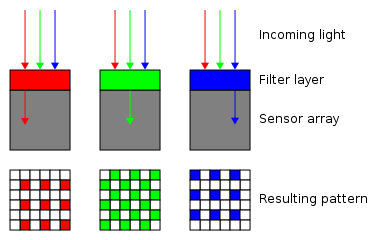
The most commonly used CFA is the Bayer filter mosaic as shown on Figure 54. The filter pattern is 50% green, 25% red and 25% blue. It should be noted that both various modifications of colours and arrangement and completely different technologies are available, such as colour co-site sampling or the Foveon X3 sensor.
3.4. Image processing
After the image acquisition with the image sensor, the image processing should be started. In computer vision systems there are some typical processing steps which generally cover the operation of the automotive cameras. In the following listing, which is based on [34], these steps are detailed complemented with the automotive specialities.
-
Pre-processing – Before a computer vision method can be applied to image data in order to extract some specific piece of information, it is usually necessary to process the data in order to assure that it satisfies certain assumptions implied by the method. Examples are
-
Re-sampling in order to assure that the image coordinate system is correct.
-
Noise reduction in order to assure that sensor noise does not introduce false information.
-
Contrast enhancement to assure that relevant information can be detected.
-
Scale space representation to enhance image structures at locally appropriate scales.
-
Feature extraction – Image features at various levels of complexity are extracted from the image data. Typical examples of such features are
-
Lines, edges. Primarily used in lane, road sign and object detection functions.
-
Localized interest points such as corners.
-
More complex features may be related to shape or motion.
-
Detection/segmentation – At some point in the processing a decision is made about which image points or regions of the image are relevant for further processing. Examples are
-
Segmentation of one or multiple image regions which contain a specific object of interest. Typically used in night vision to separate the ambient light sources from the vehicle lights.
-
High-level processing – At this step the input is typically a small set of data, for example a set of points or an image region which is assumed to contain a specific object. The remaining processing deals with, for example:
-
Verification that the data satisfy model-based and application specific assumptions.
-
Estimation of application specific parameters, such as object size, relative speed and distance.
-
Image recognition – classifying a detected object into different categories. (E.g. passenger vehicle, commercial vehicle, motorcycle.)
-
Image registration – comparing and combining two different views of the same object in stereo cameras.
-
Decision making – Making the final decision required for the application. These decisions can be classified as mentioned in Section 1.3, for example:
-
Inform about road sign
-
Warn of the lane departure
-
Support ACC with lanes, objects’ speed and distance (adding complementary information to the radar)
-
Intervene with steering or breaking in case of lane departure
3.5. Applications
The automotive cameras can be classified several ways. The most important aspects are the location (front, rear), colouring (monochrome, monochrome+1 colour, RGB) and the spatiality (mono, stereo).
The rear cameras are usually used for parking assistant functions, whilst the front cameras can provide several functions such as:
-
Object detection
-
Road sign recognition
-
Lane detection
-
Vehicle detection and environment sensing by dark for headlight control
-
Road surface quality measurement
-
Supporting and improve radar-based functions (Adaptive Cruise Control, Predictive Emergency Braking System, Forward Collision Warning)
-
Traffic jam assist, construction zone assist
The colouring capabilities influence the reliability and the precision of some camera functions. Basically most of the main functions can be implemented with a mono camera, which detects only the intensity of light on each pixel. On the other hand only one plus colour can significantly help to reach better performance. For example with red sensitive pixels the road sign recognition could be more reliable.
The mono or stereo design of the camera has strong influence on the 3D vision, which is important for measuring the distances of the objects and to detect the imperfections of the road.
To deal with the aforementioned tasks the output of the imager is processed by a high computing performance CPU-based control unit. The CPU is often supported with an FPGA which is fast enough to perform the pre-processing and feature extraction tasks.
The output of the camera can be divided into two classes, which also means two different architectures:
-
Low-level (image) interfaces: analogue, LVDS (low-voltage differential signalling)
-
High-level (identified objects description): CAN, FlexRay
In the first case the imager with the lens and the control unit are installed in different places inside the vehicle, whilst in the second case all of the necessary parts are integrated into a common housing and placed beyond the windshield. This integrative approach doesn’t require a separate control unit.
As an example of a modern automotive camera the Stereo Video Camera of Bosch has the following main properties. Its two CMOS (complementary metal oxide semiconductor) colour imagers have a resolution of 1280 x 960 pixels. Using a powerful lens system, the camera records a horizontal field of view of 45 degrees and offers a 3D measurement range of more than 50 meters. The image sensors, which are highly sensitive in terms of lighting technology, can process very large contrasts and cover the wavelength range that is visible to humans.
This stereo camera enables a variety of functions that has already been mentioned before. The complete three-dimensional recording of the vehicle's surroundings also provides the basis for the automated driving functions of the future. (Source: [35]
Compared to the aforementioned Bosch Stereo Camera the following table shows the main properties of the Continental CSF200 mono camera.
|
Range |
Maximum: 40m … 60m |
|
Sensor |
RGB 740 x 480 pixel |
|
Field of view |
horizontal coverage: 42° vertical coverage: 30° |
|
Cycle Time |
60ms |
3.6. Night Vision
The digital imaging and computer vision have become more and more important on the road towards the fully autonomous car. But the imagers in these cameras have got a hard constraint which is the absence of light. To overcome these shortcomings several night vision systems were developed in the past decades, which is summarized in the followings based on [36].
Nowadays there are two main technologies are available for the vehicle manufacturers:
-
Far Infrared (FIR) technology
-
Near Infrared (NIR) technology
An FIR system is passive, detecting the thermal radiation (wavelength of around 8–12 um). Warm objects emit more radiation in this region and thus have high visibility in the image. NIR systems use a near-infrared source to shine light with a wavelength of around 800 nm at the object and then detect the reflected illumination. The main advantage of NIR systems is that the cost is lower, because the sensor technology at these wavelengths is already well developed for other imaging applications such as video cameras. A NIR hardware can also potentially be combined with other useful functions such as lane departure warning.
In contrast, FIR systems offer a superior range and pedestrian-detection capability, but their sensors cannot be mounted behind the windscreen or other glass surfaces. University of Michigan Transport Research Institute studies comparing the ability of drivers to spot pedestrians using both the NIR and FIR devices showed that under identical conditions, the range of an FIR system was over three times further than that obtained with NIR — 119 m compared with 35 m.
|
Pros |
NIR |
Pros |
FIR |
|
Lower sensor cost |
Superior detection range |
||
|
Higher image resolution |
Emphasizes objects of particular risk for example, pedestrians and animals |
||
|
Potential for integrating into other systems |
Images with less visual clutter (unwanted features that may distract driver) |
||
|
Favourable mounting location |
Better performance in inclement weather |
||
|
Cons |
Cons |
||
|
Sensitive to glare from oncoming headlights and other NIR systems |
Lower contrast for objects of ambient temperature |
||
|
Detection range depends on reflectivity of object |
|
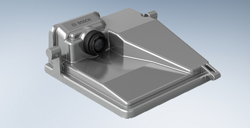
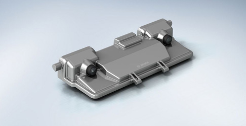
Night-vision systems were first introduced into the 2000 model of the Cadillac Deville (FIR) and thereafter by Lexus/Toyota in 2002 (NIR). In September 2005, BMW introduced the Autoliv Night Vision System [37] as an optional feature which used a thermal image sensor. featuring a 320 times 240 array of detector elements (pixels) that sense very small temperature differences in the environment (less than a tenth of a degree). The sensor, 57 x 58 x 72 mm in size excluding the connector, is mounted on the car's front bumper just below and to one side of the number plate.
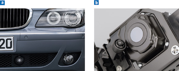
In terms of performance, the system offers a range of 300 m, a 36° field of view in the horizontal and a 30 Hz refresh rate. By using a highly sensitive FIR camera, the driver is given a clear view of the road ahead and can easily distinguish warm (living) objects that have a temperature different from that of the ambient air. For ease of use, the image is automatically optimized to preserve image quality over a range of driving conditions.
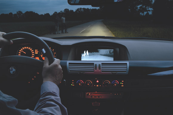
For driving speeds in excess of 70 km per hour, the image is automatically magnified 1.5 times using an electronic zoom function. An electronic panning function, which is controlled by the angle of the steering wheel, ensures that the image matches the car direction and follows the curve of the road.
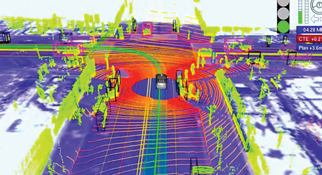
3.7. Laser Scanner (LIDAR)
Similarly to RADAR LiDAR means LIght Detection And Ranging. The main purpose of the laser scanner system is the detection and tracking of other vehicles, pedestrians and stationary objects (e.g. guard rails).
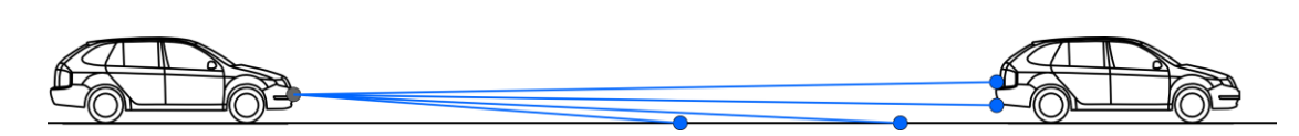
Differences between Lidars and laser scanners are detailed in the following paragraphs. The Lidar is static which means it can measure in one direction (Traffipax). Instead of radio waves used by RADAR, LIDAR uses ultra violet, visible or infrared light pulses for detection. The light pulses are sent out of the sensor in many directions simultaneously and reflected by the surrounding objects. Object distance detection is based on precise time measurement of the pulse-echo reflection. Repeated measurement can result in speed detection of the measured object.
The Laser Scanner is dynamic which means variable viewing angle. As the LIDAR measurements are taken many times with a rotating sensor in many directions, the result is a scanned planar slice. This type of measurement is called Laser Scanning. If the measurements are taken also in different angles or the sensor is moving (on top of vehicle) a complete 3D view of the surroundings can be created.
As this process can be done many times a second (5-50Hz) a real time view of the surrounding can also be created. (Source [38]
The laser scanner may also provide lane markings detection. Together with the lane marking information of the front camera this additional feature might help to provide redundant and robust lane information.
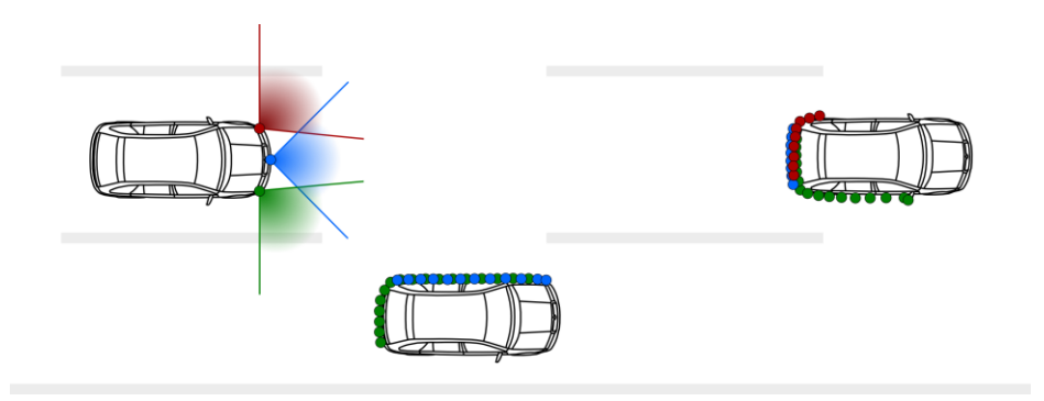
Figure 47 shows a typical laser scanner system consists of three single sensors integrated in the vehicles front bumper. One sensor is installed in the centre of the vehicle looking straight ahead. Two further sensors are integrated in the left and right front corner of the vehicle facing outwards at 30° to 40°. There is a sensor fusion algorithm that creates a complete 180 degree view to the front direction of the vehicle.
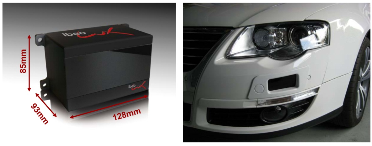
The ibeo LUX HD [39] laser scanner which is designed for reliable automotive ADAS applications and tested in project HAVEit has the following main properties.
-
Range up to 120m (30m @10% remisson)
-
All weather capability thanks to the Ibeo multi-echoe-technology: Up to 3 distance measurements per shot (allow measurements through atmospheric clutter like rain and dust)
-
Embedded object tracking
-
Wide horizontal field of view: 2 layers: 110° (50° to - 60°), 4 layers: 85° (35° to -50°)
-
Vertical field of view: 3.2°
-
Multi-layer: 4 parallel scanning layers
-
Data update rate: 12.5/ 25.0/ 50.0 Hz
-
Operating temperature range: -40 to 85 deg C
-
Accuracy (distance independent): 10 cm
-
Angular resolution:
-
Horizontal: up to 0.125°
-
Vertical: 0.8°
-
Distance Resolution: 4 cm
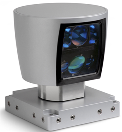
Another important product is the Velodyne HDL-64E S2 [40] laser scanner. It is designed for obstacle detection and navigation of autonomous ground vehicles and marine vessels. Its durability, 360° field of view and very high data rate makes this sensor ideal for the most demanding perception applications as well as 3D mobile data collection and mapping applications. This laser scanner is used in Google’s driverless car project.
-
905 nm wavelength, 5 ns pulses
-
15V 4A
-
Ethernet output
-
less than 2 cm accuracy
-
Max 15 Hz update rate (900RPM)
-
Range 120m
-
0.09 degree of vertical resolution
-
26 degree of vertical field of view
-
More than 1.3 million points detected per second
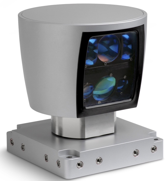
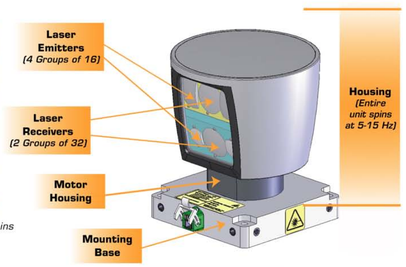
Typical components of a laser scanner sensor are the following:
-
Laser source (emitters)
-
Scanner optics
-
Laser detector (receivers)
-
Control electronics
-
Position and navigation systems
The general architecture of the laser scanners is shown in Figure 51.
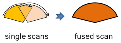
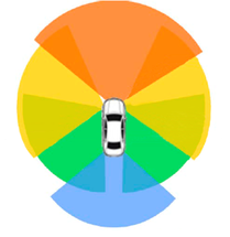
Should the horizontal aperture angle be not enough for a specific application that requires a greater field of vision, there is fusion scan available. Up to six sensors can be combined together. The data of the individual sensors are synchronized and combined together using a special software, resulting in one fused scan. With laser scanner fusion there is a possibility to achieve a seamless 360 degrees scanning of the vehicle's surroundings.
3.8. eHorizon
The so-called eHorizon is an integrated information source including map information, route information, speed limit information, 3D landscape data, positioning and navigation information (GPS, GLONASS, etc.) for the advanced driver assistance systems (ADAS) within the car. With the help of this information the forward thinking driving function can be improved (e.g. predictive control considering road inclinations and speed limits) and the fuel consumption can be decreased.
3.8.1. NAVSTAR GPS
The Navigation Signal Timing and Ranging Global Positioning System (NAVSTAR GPS, in short GPS) is a U.S. government owned utility that provides users with positioning, navigation, and timing (PNT) services. The following summary of the operating principles is based on [41].
This system consists of three segments: the space segment, the control segment, and the user segment. The U.S. Air Force develops, maintains, and operates the space and control segments.
The space segment consists of a constellation of satellites transmitting radio signals to users. The United States is committed to maintaining the availability of at least 24 operational GPS satellites, 95% of the time. To ensure this commitment, the Air Force has been flying 31 operational GPS satellites for the past few years. The extra satellites may increase GPS performance but are not considered part of the core constellation. GPS satellites fly in medium Earth orbit (MEO) at an altitude of approximately 20,200 km. Each satellite circles the Earth twice a day. The satellites in the GPS constellation are arranged into six equally-spaced orbital planes surrounding the Earth. Each plane contains four "slots" occupied by baseline satellites. This 24-slot arrangement ensures users can view at least four satellites from virtually any point on the planet.
The control segment consists of a global network of ground facilities that track the GPS satellites, monitor their transmissions, perform analyses, and send commands and data to the constellation. The current operational control segment includes a master control station, an alternate master control station, 12 command and control antennas, and 16 monitoring sites.
The user segment consists of the GPS receiver equipment, which receives the signals from the GPS satellites and uses the transmitted information to calculate the user’s three dimensional position and time.
The GPS satellites broadcast radio signals providing their locations, status, and precise time (t1) from on-board atomic clocks.
The principle of the operation is based on distance measurement. The GPS satellites broadcast radio signals providing their locations, status, and precise time from on-board atomic clocks. The GPS radio signals travel through space at the speed of light. A GPS device receives the radio signals, noting their exact time of arrival, and uses these to calculate its distance from each satellite in view. To calculate its distance from a satellite, a GPS device applies this formula to the satellite's signal:
distance = rate x time
where rate is the speed of light and time is how long the signal travelled through space
(This requires quite precise time measurement, since 1 us time deviation would result in 300m distance deviation.) The signal's travel time is the difference between the time broadcast by the satellite and the time the signal is received.
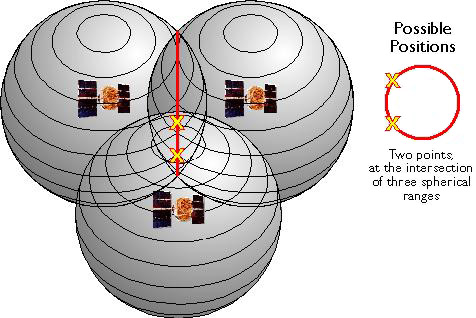
If distances from three satellites are known, the receiver's position must be one of two points at the intersection of three spherical ranges (see Figure 54). GPS receivers are usually smart enough to choose the location nearest to the Earth's surface. At a minimum, three satellites are required for a two-dimensional (horizontal) fix if our receiver’s clock would be perfect. In this theoretical case all our satellite ranges would intersect at a single point (which is our position). But with imperfect clocks, a fourth measurement, done as a cross-check, will not intersect with the first three. Since any offset from universal time will affect all of our measurements, the receiver looks for a single correction factor that it can subtract from all its timing measurements that would cause them all to intersect at a single point. That correction brings the receiver's clock back into sync with universal time. Once it has that correction it applies to all the rest of its measurements and now we've got precise positioning. One consequence of this principle is that any decent GPS receiver will need to have at least four channels so that it can make the four measurements simultaneously.
The modernization program of the GPS was started in May 2000 with turning off the GPS Selective Availability (SA) feature. SA was an intentional degradation of civilian GPS accuracy, implemented on a global basis through the GPS satellites. During the 1990s, civil GPS readings could be incorrect by as much as a football field (100 meters). On the day SA was deactivated, civil GPS accuracy improved tenfold, benefiting civil and commercial users worldwide. In 2007, the government announced plans to permanently eliminate SA by building the GPS III satellites without it. The GPS modernization program involves a series of consecutive satellite acquisitions. It also involves improvements to the GPS control segment, including the Architecture Evolution Plan (AEP) and the Next Generation Operational Control System (OCX). The main goal is to improve GPS performance using new civilian and military signals. In addition GPS modernization is introducing modern technologies throughout the space and control segments that will enhance overall performance. For example, legacy computers and communications systems are being replaced with a network-centric architecture, allowing more frequent and precise satellite commands that will improve accuracy for everyone.
From the point of view of the transportation the Second and the Third Civil Signals (L2C and L5) will be the most significant changes in the modernized GPS system. L2C is designed specifically to meet commercial needs. When combined with L1 C/A in a dual-frequency receiver, L2C enables ionospheric correction, a technique that boosts accuracy. Civilians with dual-frequency GPS receivers enjoy the same accuracy as the military (or better). For professional users with existing dual-frequency operations, L2C delivers faster signal acquisition, enhanced reliability, and greater operating range. L2C broadcasts at a higher effective power than the legacy L1 C/A signal, making it easier to receive under trees and even indoors.
L5 is designed to meet demanding requirements for safety-of-life transportation and other high-performance applications. L5 is broadcast in a radio band reserved exclusively for aviation safety services. It features higher power, greater bandwidth, and an advanced signal design. Future aircraft will use L5 in combination with L1 C/A to improve accuracy (via ionospheric correction) and robustness (via signal redundancy). In addition to enhancing safety, L5 use will increase capacity and fuel efficiency within U.S. airspace, railroads, waterways, and highways.
Both signals are in launching phase. The L2C will be available on 24 GPS satellites around 2018 and the L5 around 2021.
3.8.2. GLONASS
GLONASS (Globalnaya Navigatsionnaya Sputnikovaya Sistema or Global Navigation Satellite System) is a GNSS operated by the Russian Aerospace Defence Forces. Development of GLONASS began in 1976, with a goal of global coverage by 1991 [42]. Beginning on 12 October 1982, numerous rocket launches added satellites to the system until the constellation was completed in 1995. GLONASS was developed to provide real-time position and velocity determination, initially for use by the Soviet military in navigating and ballistic missile targeting. With the collapse of the Russian economy GLONASS rapidly degraded, mainly due to the relatively short design life-time of the GLONASS satellites. Beginning in 2001, Russia committed to restoring the system, and in recent years has diversified, introducing the Indian government as a partner. This plan calls for 18 operational satellites in orbit by 2008 and 24 satellites (21 operational and 3 on-orbit spares deployed in three orbital planes) in place by 2009; and a level of performance matching that of the U.S Global Positioning System by 2011. Finally by 2010, GLONASS has achieved 100% coverage of Russia's territory and in October 2011, the full orbital constellation of 24 satellites was restored, enabling full global coverage. It both complements and provides an alternative to the United States' Global Positioning System (GPS) and is the only alternative navigational system in operation with global coverage and of comparable precision.
At present GLONASS provides real time position and velocity determination for military and civilian users. The fully operational GLONASS constellation consists of 24 satellites, with 21 used for transmitting signals and three for in-orbit spares, deployed in three orbital planes. The three orbital planes' ascending nodes are separated by 120° with each plane containing eight equally spaced satellites. The orbits are roughly circular, with an inclination of about 64.8°, and orbit the Earth at an altitude of 19,100 km, which yields an orbital period of approximately 11 hours, 15 minutes. The planes themselves have a latitude displacement of 15°, which results in the satellites crossing the equator one at a time, instead of three at once. The overall arrangement is such that, if the constellation is fully populated, a minimum of 5 satellites are in view from any given point at any given time. This guarantees for continuous and global navigation for users world-wide.
3.8.3. Galileo
Galileo is Europe’s own global navigation satellite system, providing a highly accurate, guaranteed global positioning service under civilian control, which is introduced from [43].
By offering dual frequencies as standard, Galileo will deliver real-time positioning accuracy down to the metre range. It will guarantee availability of the service under all but the most extreme circumstances and will inform users within seconds of any satellite failure, making it suitable for safety-critical applications such as guiding cars, running trains and landing aircraft. On 21 October 2011 came the first two of four operational satellites designed to validate the Galileo concept in both space and on Earth. Two more followed on 12 October 2012. This In-Orbit Validation (IOV) phase is now being followed by additional satellite launches to reach Initial Operational Capability (IOC) by mid-decade.
Galileo services will come with quality and integrity guarantees, which mark the key difference of this first complete civil positioning system from the military systems that have come before. A range of services will be extended as the system is built up from IOC to reach the Full Operational Capability (FOC) by this decade’s end. The fully deployed Galileo system consists of 30 satellites (27 operational + 3 active spares), positioned in three circular Medium Earth Orbit (MEO) planes at 23 222 km altitude above the Earth, and at an inclination of the orbital planes of 56 degrees to the equator.
The four operational satellites launched so far - the basic minimum for satellite navigation in principle - serve to validate the Galileo concept with both segments: space and related ground infrastructure. On March 12th, 2013, a first positioning test based on the 4 first operational Galileo satellites was conducted by ESA. This first position fix returned an accuracy range of +/- 10 meters, which is considered as very good, considering that only 4 satellites (out of the total constellation of 30) are already deployed. The Open Service, Search and Rescue and Public Regulated Service will be available with initial performances soon. Then as the constellation is built-up beyond that, new services will be tested and made available to reach Full Operational Capability (FOC). Once this is achieved, the Galileo navigation signals will provide good coverage even at latitudes up to 75 degrees north, which corresponds to Norway's North Cape - the most northerly tip of Europe - and beyond. The large number of satellites together with the carefully-optimised constellation design, plus the availability of the three active spare satellites, will ensure that the loss of one satellite has no discernible effect on the user.
3.8.4. BeoiDou (COMPASS)
The BeiDou Navigation Satellite System (BDS) is a Chinese satellite navigation system. It consists of two separate satellite constellations – a limited test system that has been operating since 2000, and a full-scale global navigation system that is currently under construction.
The first BeiDou system, officially called the BeiDou Satellite Navigation Experimental System and also known as BeiDou-1, consists of three satellites and offers limited coverage and applications. It has been offering navigation services, mainly for customers in China and neighbouring regions, since 2000.
The second generation of the system officially called the BeiDou Satellite Navigation System (BDSNS) and also known as COMPASS or BeiDou-2, will be a global satellite navigation system. According to the plans the full constellation will consist of 35 satellites. Since December 2012 there are 10 satellites providing local services to the Asia-Pacific area and it is planned to cover all over the world serving global customers before 2020. [44]

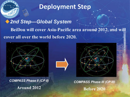
The COMPASS Phase II has successfully established as planned. On December 27, 2013, the first anniversary of BeiDou Navigation Satellite System providing full operational regional service was held in Beijing. At the meeting, China Satellite Navigation System Management Office Director Ran Chengqi announced the BeiDou Navigation Satellite System Public Service Performance Standard.
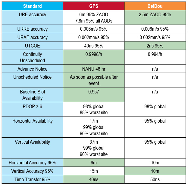
The result comparison with GPS created by John Lavrakas (Advanced Research Corporation) [45] shows mixed results. In some cases, the commitments from BeiDou were stronger (URE accuracy, the table to show green for the GNSS service committing to a more stringent standard over the other vertical position), and in other cases the commitments from GPS were stronger (continuity of service, advance notice of outages).
3.8.5. Differential GPS
Differential correction techniques are used to enhance the quality of location data gathered using global positioning system (GPS) receivers. Differential correction can be applied either in real-time (directly in the field, during measurement) or when post-processing data in the office (later during data evaluation). Although both methods are based on the same underlying principles, each accesses different data sources and achieves different levels of accuracy. Combining both methods provides flexibility during data collection and improves data integrity.
The underlying assumption of differential GPS (DGPS) technology is that any two receivers that are relatively close together will experience similar atmospheric errors. DGPS requires that one GPS receiver must be set up on a precisely known location. This GPS receiver is the base or reference station. The base station receiver calculates its position based on satellite signals and compares this location to the already known precise location resulting in a difference. This difference then is applied to the GPS data recorded by the second GPS receiver, which is known as the roving receiver. The corrected information can be applied to data from the roving receiver in real time in the field using radio signals or through post-processing after data capture using special processing software.
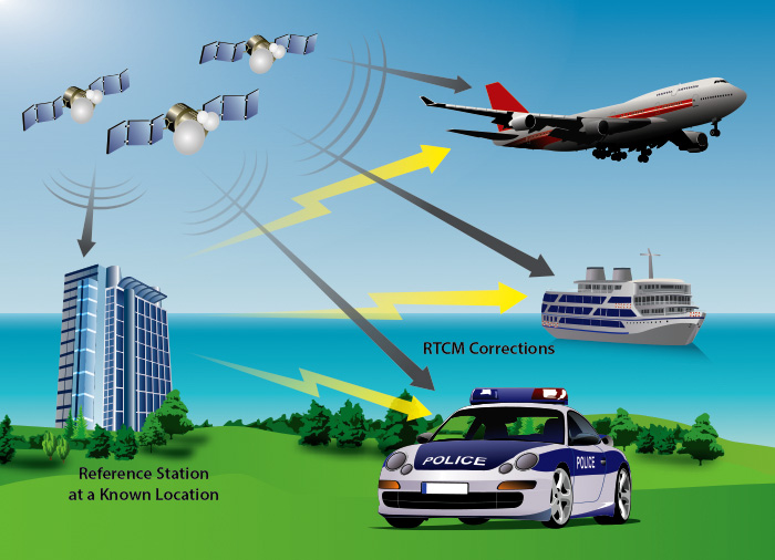
Real-time DGPS occurs when the base station calculates and broadcasts corrections for each satellite as it receives the data. The correction is received by the roving receiver via a radio signal if the source is land based or via a satellite signal if it is satellite based and applied to the position it is calculating. As a result, the position displayed and logged to the data file of the roving GPS receiver is a differentially corrected position.
In the US, the most widely available DGPS system is the Wide Area Augmentation System (WAAS). The WAAS was created by the Federal Aviation Administration and the Department of Transportation for use in precision flight approaches. However, the system is not limited to aviation applications, and many of the commercial GPS receivers intended for maritime and automotive use support WAAS. WAAS provides GPS correction data across North America with a typical accuracy less than 5 meters. Similar systems are available in Europe.
The European Geostationary Navigation Overlay Service (EGNOS) is the first pan-European satellite navigation system. It augments the US GPS satellite navigation system and makes it suitable for safety critical applications such as flying aircraft or navigating ships through narrow channels.
Consisting of three geostationary satellites and a network of ground stations, EGNOS achieves its aim by transmitting a signal containing information on the reliability and accuracy of the positioning signals sent out by GPS. It allows users in Europe and beyond to determine their position to within 1.5 meters. (Source: [46])
Another high precision GPS solution is the real-time kinematic GPS (RTK GPS). RTK is a GBS-based survey that utilizes a fixed, nearby ground base station that is in direct communication with the rover receiver through a radio link. RTK is capable of taking survey grade measurements in real time and providing immediate accuracy to within 1-5 cm. RTK systems are the most precise of all GNSS systems. They are also the only systems that can achieve complete repeatability, allowing the returning to the exact location indefinitely. All this precision and repeatability comes at a fairly high cost. But there are other drawbacks to RTK also. RTK requires a base station within about 10-15 km of the rover. [47]
3.8.6. Assisted GPS
Assisted GPS describes a system where outside sources, such as an assistance server and reference network, help a GPS receiver perform the tasks required to make range measurements and position solutions. The assistance server has the ability to access information from the reference network and also has computing power far beyond that of the GPS receiver. The assistance server communicates with the GPS receiver via a wireless link (generally mobile network data link). With assistance from the network, the receiver can operate (start-up) more quickly and efficiently than it would unassisted, because a set of tasks that it would normally handle is shared with the assistance server. The resulting AGPS system, consisting of the integrated GPS receiver and network components, boosts performance beyond that of the same receiver in a stand-alone mode. It improves the start-up performance or time-to-first-fix (TTFF) of the GPS receiver. The assistance server is also able to compute position solutions, leaving the GPS receiver with the sole job of collecting range measurements. The only disadvantage of AGPS is that it depends on the infrastructure (requiring an assistant service and an on-line data connection). (Source: [48])
3.9. Data Fusion
The data fusion is responsible for comparing all relevant sensor information, carrying out feasibility increasing the reliability of the individual sensor information and increasing precision of the sensor information. The data fusion provides all necessary information to the following command layer in order to be able to complete its task successfully.
The Data Fusion harmonizes the on-board environment sensor signal, the vehicle sensor signals (vehicle speed, yaw rate, steering angle, longitudinal, lateral acceleration, etc.) The output of the sensor fusion is the vehicle status (Position and kinematic state information); and environmental status (position and shape of the surrounding objects including the vehicle in front of us). The environmental objects can also be classified into categories be means of dimension and type of objects.
-
Front vehicle
-
Surrounding objects (obstacles)
-
Lane information
-
Road information
-
Intersection information
-
Trip information
Sensor data fusion calculates an overall environment perception taking the information of all sensors into account.
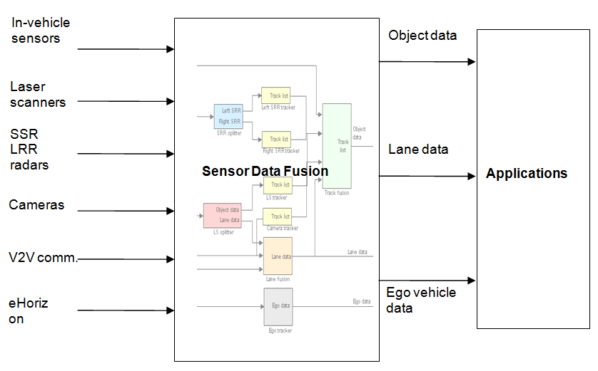
Sensor data fusion is generally a separate module inside the vehicle control system. It receives data from many sources, including in-vehicle sensors, environment monitoring sensors (radar, laser and camera), V2V communication, eHorizon, etc. The environment sensors are heterogeneous sources of information, providing data describing surrounding objects and road. Each sensor makes different estimates of the environment properties, using both overlapping and independent fields of view. Moreover, each of these sources transmits data in its own spatial and temporal format.
The sensor data fusion gathers sensor data and executes several tasks in order to provide useful estimates which are synchronized and spatially aligned. The synchronised and spatially aligned data, called the perception model, is then available for Highly Automated Driving applications. The perception model consists of state estimations of relevant objects, the road and a refined ego vehicle state.
To achieve the synchronized and spatially aligned view of the environment, the sensor data fusion will make use of several algorithms and filters to provide high level output data.
There are several sensors measuring the same objects surrounding the vehicle (laser scanners, short and long range radars, mono and colour cameras, V2V communication). Each sensor measures different aspects of an object, for example, the laser scanners measure both position and velocity, whereas the camera simply estimates object position. Therefore each sensor data have to be evaluated and filtered first to reach a common (homogenous) object representation, then comes the effective fusion of the data.
There are several algorithms exist for sensor data fusion, such as Cross-Covariance Fusion, Information Fusion, Maximum A-Posterior Fusion and Covariance Fusion.
The standardized output state for each detected object contains the following information:
-
Position
-
Vehicle Speed and Acceleration)
-
Object Size
-
Object Classification (tree, vehicle, pedestrian, etc.)
-
Output Data Confidence Level