Chapter 6. Fuzzy automaton for describing ethological functions

In recent years there has been an increased interest in the development of Human-Robot Interaction (HRI). Researchers have assumed that HRI could be enhanced if these intelligent systems were able to express some pattern of sociocognitive and socioemotional behaviour (e.g. REF _Ref361667391 \r \h \* MERGEFORMAT ). Such approach needed an interaction among various scientific disciplines including psychology, cognitive science, social sciences, artificial intelligence, computer science and robotics. The main goal has been to find ways in which humans can interact with these systems in a ‘natural’ way. Recently HRI has become very user oriented, that is, the performance of the robot is evaluated from the user’s perspective. This view also reinforces arguments that robots do not only need to display certain emotional and cognitive skills but also showing features of individuality. Generally however, most socially interactive robots are not able to support long-term interaction with humans, and the interest shown toward them wears out rapidly.

The design of socially interactive robots has faced many challenges. Despite major advances there are still many obstacles to be solved in order to achieve a natural-like interaction between robots and humans. The ‘uncanny valley’ effect: Mori REF _Ref361656179 \r \h \* MERGEFORMAT assumed that the increasing similarity of robots to humans will actually increase the chances that humans refuse interaction (will be frightened from) very human-like agents. Although many take this effect for granted only little actual research was devoted to this issue. Many argue that once an agent passes certain level of similarity, as it is the case in the most recent visual characters in computer graphics, people will treat them just as people REF _Ref361667499 \r \h \* MERGEFORMAT . However, in the case of 3D robots, the answer is presently less clear, as up do date technology is very crude in reproducing natural-like behaviour, emotions and verbal interaction. Thus for robotics the uncanny valley effect will present a continuing challenge in the near future.

In spite of the huge advances in robotics current socially interactive systems fail both with regard to motor and cognitive capacities, and in most cases can interact only in a very limited way with the human partner. This is a major discrepancy that is not easy to solve because there is a big gap between presently available technologies (hardware and software) and the desire for achieving human-like cognitive and motor capacities. As a consequence recent socially interactive robots have only a restricted appeal to humans, and after losing the effect of novelty the interactions break down fast.

The planning and construction of biologically or psychologically inspired robots depends crucially of the current understanding of human motor and mental processes. However, these are one of the most complex phenomena of life. Therfore it is certainly possible that human mental models of abilities like ‘intention’, ‘human memory’ etc., which serve at present as the underlying concepts for control socially interactive robots, will be proved to be faulty.

Because of the goal of mimicking a human, socially interactive robots do not utilize more general human abilities that have evolved as general skills for social interaction. Further, the lack of evolutionary approach in conceptualizing the design of such robots hinders further development, and reinforces that the only goal in robotics should be the produce ‘as human-like as possible’ agents.

In order to overcome some of the challenges presented above ethologically inspired HRI models can be applied. The concept of ethologically inspired HRI models allows the study of individual interactions between animals and animals and humans. This way of handling Human-Robot Interaction is based on the concept that the robot acts like an animal companion to human. According to this paradigm the robot should not be molded to mimic the human being, and form human-to-human like communication, but to follow the existing biological examples and form inter-species interaction. The 20.000 year old human-dog relationship REF _Ref361667925 \r \h \* MERGEFORMAT is a good example for this paradigm of the HRI, as interaction of different species. One good reason of this approach in HRI is the lack of the ‘uncanny valley’ effect REF _Ref361656179 \r \h \* MERGEFORMAT , i.e. there is no need to buit robots which have any similarities to humans.

Such robots do not have to rely on the exact copy of human social behaviour (including language, etc.) but should be able to produce social behaviours that provide a minimal set of actions on which human-robot cooperation can be achieved. Such basic models of robots could be improved with time making the HRI interaction more complex.

In ethological modeling, mass of expert knowledge exists in the form of expert’s rules. Most of them are descriptive verbal ethological models. The knowledge representation of an expert’s verbal rules can be very simply translated to the structure of fuzzy rules, transforming the initially verbal ethological models to a fuzzy model. On the other hand, in case of the descriptive verbal ethological models, the ‘completeness’ of the rule-base is not required (thanks to the descriptive manner of the model), which makes implementation difficulties in classical fuzzy rule based systems. For that reason for fuzzy modell we use low computational demand Fuzzy Rule Interpolation (FRI) methods like FIVE REF _Ref385680017 \r \h . The application of FRI methods fits well the conceptually sparse rule-based (‘incomplete’) structure of the existing descriptive verbal ethological models.

The main benefit of the FRI method adaptation in ethological model implementation is the fact, that it has a simple rule-based knowledge representation format. Because of this, even after numerical optimization of the model, the rules remain ‘human readable’, and helps the formal validation of the model by the ethological experts. On the other side due to the FRI base, the model has still low computational demand and fits directly the requirements of the embedded implementations.

For implementing ethologically inspired HRI models the classical behaviour-based control structure is suggested, described in the followings.

The main building blocks of Behaviour-based Control (BBC, a comprehensive overview can be found in REF _Ref358152640 \r \h ) are the behaviour components themselves. The behaviour components can be copies of typical human or animal behaviors, or can be artificially created behaviours. The actual behaviour response of the system can be formed as one of the existing behaviour component, which gives the best match to the actual situation, or a fusion of the behaviour components based on their suitability for the actual situation. Encoding the behaviour components can be realized with e.g. simple reflexive agents, which assign an output response to each input situation.

In case when more than one behaviour components are simultaneously competing for the same ‘actuator’ the aggregation or selection of the behaviour components is necessary. Handling multiple behaviour components in a BBC system can be done in two ways. The first is the competitive way, when the behaviour components are assigned with priorities, and the behaviour component with the highest priority takes precedence, while the behaviours with lower priorities are simply ignored. The second is the cooperative way when the outputs are fusioned based on various criteria.

This structure has two main tasks. The first is a decision of which behaviour is needed in an actual situation, and the levels of their necessities in case of behaviour fusion. The second is the way of the behaviour fusion. The first task can be viewed as an actual system state approximation, where the actual system state is the set of the necessities of the known behaviours needed for handling the actual situation. The second is the fusion of the known behaviours based on these necessities. In case of the suggested fuzzy behaviour based control structures both tasks are solved by FRI systems. If the behaviours are also implemented on FRI models, the behaviours together with the behaviour fusion modules form a hierarchical FRI system.

The application of FRI methods in direct fuzzy logic control systems gives a simplified way for constructing the fuzzy rule base. The rule base of a fuzzy interpolation-based model, is not necessarily complete, it could contain the most significant fuzzy rules only without risking the chance of having no conclusion for some of the observations. The model always gives a usable conclusion even if there are no rules defined for the actual observations. In other words, during the construction of the fuzzy model, it is enough to concentrate on the main actions (rules could be deduced from the others could be intentionally left out from the model, radically simplifying the rule base creation, saving time consuming work.).

For demonstrating the main benefits of the FRI model in behaviour-based control, here the focus is only on the many cases most heuristic part of the structure, on the behaviour coordination. The task of behaviour coordination is to determine the necessities of the known behaviours needed for handling the actual situation.

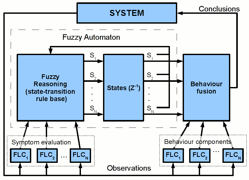
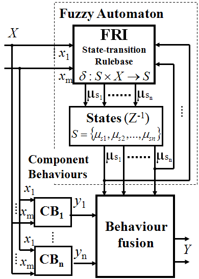
In the suggested behaviour-based control structure for achieving the decision related to the relevance of the behaviour components this work adapts the concept of the finite state fuzzy automaton REF _Ref361677815 \r \h \* MERGEFORMAT (see Fig. 6-1 and the next chapter for more details), where the state of the finite state fuzzy automaton is the set of the suitabilities of the component behaviours. This solution is based on the heuristic, that the necessities of the known behaviours for handling a given situation can be approximated by their suitability. And the suitability of a given behaviour in an actual situation can be approximated by the similarity of the situation and the prerequisites of the behaviour. (Where the prerequisites of the behaviour is the description of the situations where the behaviour is applicable). This case instead of determining the necessities of the known behaviours, the similarities of the actual situation to the prerequisites of all the known behaviours can be approximated.

The system consists (see Fig. 6-1) of not only the fuzzy automaton but the behaviour fusion component and various component behaviours implemented on fuzzy logic controllers (FLC). The state variables characterize the relevance of the component behaviours. The state-transition rule base of the automaton applies fuzzy rule interpolation for state-transition evaluation. The previous states are fed back to the automaton and the conclusion given by the automaton is used as weights in the behaviour fusion component for determining the final conclusion of the BBC. The conclusion of the fuzzy automaton will be the new system state for the next step of the behaviour fusion. The behaviour fusion component can be also implemented by fuzzy reasoning (e.g. using fuzzy rule interpolation), or simply as a weighted sum. The symptom evaluation (from the terminology of fault classification) components provide a kind of preprocessing for the automaton based on the gathered observations. These components also can employ FRI techniques.

Therefore the first step of the system state approximation is determining the similarities of the actual situation to the prerequisites of all the known behaviours. The task of symptom evaluation is basically a series of similarity checking between an actual symptom (observations of the actual situation) and a series of known symptoms (the prerequisites – symptom patterns – of the behaviour components). These symptom patterns are characterizing the systems states where the corresponding behaviours are valid. Based on these patterns, the evaluation of the actual symptom is done by calculating the similarity values of the actual symptom (representing the actual situation) to all the known symptoms patterns (the prerequisites of the known behaviours). There are many existing methods for fuzzy logic symptom evaluation. For example fuzzy classification methods e.g. the Fuzzy c-Means fuzzy clustering algorithm REF _Ref361758798 \r \h can be adopted, where the known symptoms patterns are the cluster centers, and the similarities of the actual symptom to them can be fetched from the fuzzy partition matrix. On the other hand, having a simple situation, the fuzzy logic symptom evaluation could be an FRI model too.

One of the main difficulties of the system state approximation is the fact, that most cases the symptoms of the prerequisites of the known behaviours are strongly dependent on the actual behaviour of the system. Each of the behaviours has its own symptom structure. In other words, for the proper system state approximation the approximated system state is needed itself. A very simple way of solving this difficulty is the adaptation of fuzzy automaton. This case the state vector of the automaton is the approximated system state, and the state-transitions are driven by fuzzy reasoning (‘Fuzzy Reasoning (state-transition rule base)’ on Fig. 6-1), as a decision based on the previous actual state (the previous iteration step of the approximation) and the results of the symptom evaluation.

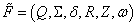
As mentioned previously, the structure of the proposed model follows the behavior-based control concept REF _Ref358152640 \r \h , i.e. the actual behavior of the system is formed as a fusion of the known component behaviors appeared to be the most appropriate in the actual situation. For behavior coordination in the applied model the concept of the ‘Fuzzy Automaton’ is adapted. Numerous versions and understanding of the fuzzy automaton can be found in the literature (a good overview can be found in REF _Ref286655753 \r \h ). The most common definition of Fuzzy Finite-state Automaton (FFA, summarized in REF _Ref286655753 \r \h ) is defined by a tuple (according to REF _Ref363657503 \r \h , REF _Ref286655753 \r \h and REF _Ref288780404 \r \h ):

where Q is a finite set of states, Q={q1,q2,...,qn}, Σ is a finite set of input symbols, Σ={a1,a2,...,am}, is the (possibly fuzzy) start state of , Z is a finite set of output symbols, Z={b1,b2,...,bn}, 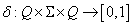is the fuzzy transition function which is used to map a state (current state) into another state (next state) upon an input symbol, attributing a value in the fuzzy interval [0,1] to the next state, and is the output function which is used to map a (fuzzy) state to the output.

Extending the concept of FFA from finite set of input symbols to finite dimensional input values turns to the following:

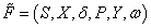
where S is a finite set of fuzzy states, 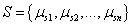, X is a finite dimensional input vector, , is the fuzzy start state of , Y is a finite dimensional output vector, , is the fuzzy state-transition function which is used to map the current fuzzy state into the next fuzzy state upon an input value, and is the output function which is used to map the fuzzy state and input to the output value. See e.g. on Fig. 6-2.

In case of fuzzy rule based representation of the state-transition function , the rules have dimensional antecedent space, and n dimensional consequent space. Applying classical fuzzy reasoning methods, the complete state-transition rule base size can be approximated by the following formula:

where n is the length of the fuzzy state vector S, m is the input dimension, i is the number of the term sets in each dimensions of the state vector, and j is the number of the term sets in each dimensions of the input vector.

According to (6.3) the state-transition rule-base size is exponential with the length of the fuzzy state vector and the number of the input dimensions. Applying FRI methods for the state-transition function fuzzy model can dramatically reduce the rule base size. See e.g. REF _Ref358152171 \r \h , where the originally exponential sized state-transition rule base of a simple heuristical model turned to be polynomial thanks to the FRI.

In case of direct application of the suggested FRI based Fuzzy Automaton for behavior-based control structures, the output function can be decomposed to parallel component behaviors and an independent behavior fusion. In this case the structure of the above introduced fuzzy automaton can turn to a very similar form as it is expected in behavior-based control (see Fig. 6-3 and Fig. 6-1). Some more details of the model implementation can be found in REF _Ref366247252 \r \h , REF _Ref366247254 \r \h and REF _Ref366247256 \r \h .

The ethological test procedure presented here has been developed for studying the affiliative relationship between a dog and its owner. The procedure is made up from seven episodes, each lasting 2 minutes, where the dog is in different situations: first with the owner, then with a stranger, or alone (according to a pre-defined protocol). Through the test, the dog’s behavior is evaluated mainly focusing on dogs’ responses related to their proximity seeking with the owner REF _Ref307389263 \r \h .

In the first episode of the test, the dog and the owner are in the test room. First the owner is passive, and then he/she stimulates playing. The second episode is where the stranger comes into the room and starts to stimulate play with the dog. Then the owner leaves the room, so in the third episode the dog is separated from the owner; the stranger tries to play with the dog then sits for a while and offers petting. The owner comes back in the beginning of the fourth episode, this is the first reunion. Meanwhile the stranger leaves the room and the dog is with the owner for two minutes. Then the owner also leaves, so in the fifth episode the dog is alone in the room. In the next episode the stranger returns and tries to stimulate playing or comfort the dog by petting it. The returning of the owner marks the beginning of the last episode. The stranger leaves the room, the owner interacts with the dog for two minutes and the test ends.

During evaluation, ethologists record pre-defined behavioral variables for describing the dogs’ responses related to both the owner and the stranger and they analyze data to reveal significant differences in behaviors showed towards the two persons.

This complex ethological model has been implemented based on the presented structure. The agent controlled by the model is the representation of the dog, other participants in the test are behaving according to a programmed scenario or are controlled by a human operator. This agent can execute a set of behaviours (moving towards specified objects, pick up or drop the toy object, wag its tail, etc.), some of them can be active and executed in parallel in the same time, but most of them are blocking each other, this latter situation is handled by the behaviour fusion component.

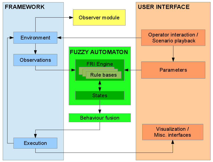
The model is basically designed for simulating the dog’s behaviour in the test described in REF _Ref307389263 \r \h \* MERGEFORMAT , but the model is flexible enough to react in an ethologically correct way for arbitrary situations. A simplified block diagram of the structure of a possible simulation framework is shown in Fig. 6-4.

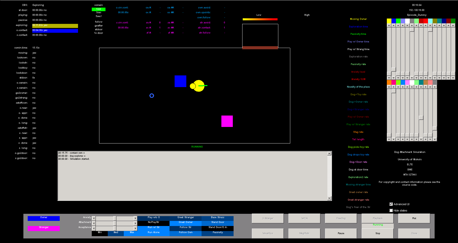
A screenshot of a possible simulation framework is shown in Fig. 6-5, where a room can be seen viewed from above, where the interactions take place. The humans are symbolized with squares, the blue square represents the owner of the dog, the magenta square represents a human unfamiliar (stranger) to the dog. The dog is represented by two circles, the large circle is the body of the dog, the smaller circle is the head of the dog, which is useful for visualizing the direction of the dog A thin green line on the dog’s body represents the tail of dog, which can change its length and also its angle (tail wagging). The color of the dog is dynamically changing showing the actual anxiety level of the dog. The room has a door where the human participants can leave or enter the room, the dog cannot go outside. Also a toy object is present (small blue circle, with a hole inside), which can be picked up and dropped by all the participants.

In the followings some example behaviours from the system and their definitions are presented.

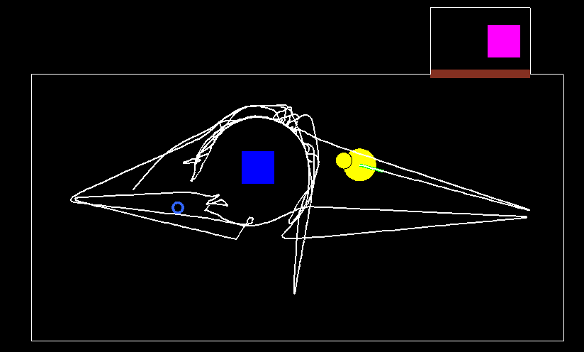
The first example behaviour set is built upon two separate component behaviours, namely ‘DogExploresTheRoom’ and ‘DogGoesToDoor’. The ‘DogExploresTheRoom’ is an exploration dog activity, in which the dog ‘looks around’ in an unknown environment (see the track marked with white in Fig. 6-6). The ‘DogGoesToDoor’ is a simple dog activity, in which the dog goes to the door, and than stands (sits) in front of it (waiting for its owner to show up again). The definition of the related state-transition FRI rules of the fuzzy automaton acts as behaviour coordination in this example.

The states concerned are the following:

As a possible rule base structure for the state-transitions of the fuzzy automaton, the following is defined (considering only the states and behaviours for this example):

If OwnerInTheRoom=False Then DogMissTheOwner=Increasing

If OwnerInTheRoom=True Then DogMissTheOwner=Decreasing

If OwnerToDogDistance=Small And Human2ToDogDistance=High Then DogAnxietyLevel=Decreasing

If OwnerToDogDistance=High And Human2ToDogDistance=LowThen DogAnxietyLevel=Increasing

State-transition rules related to the going to the door mood (state) of the Dog:

If OwnerInTheRoom=False And DogMissTheOwner=High Then DogGoesToDoor=High

If OwnerInTheRoom=True Then DogGoesToDoor=Low

State-transition rules related to the room exploration mood (state) of the Dog:

If DogAnxietyLevel=Low And OwnerStartsGame=False And ThePlaceIsUnknown=High Then DogExploresTheRoom=High

If ThePlaceIsUnknown=Low Then DogExploresTheRoom=Low

If DogAnxietyLevel=High Then DogExploresTheRoom=Low

The text in italic represent the linguistic terms (fuzzy sets) of the FRI rule base.

Also it should be noted that the rule base is sparse, containing the main state-transition FRI rules only.

A sample run of the example is introduced in Fig. 6-6 and in Fig. 6-7. At the beginning of the scene, the owner is in the room and the stranger is outside. The place is unknown for the dog (‘ThePlaceIsUnknown=High’ in the rule base). According to the above rule base, the dog starts to explore the room (see Fig. 6-6). After a little while the owner of the dog leaves the room, and then the stranger enters and stays inside (dashed white tracks in Fig. 6-7). As an effect of the changes (according to the above state-transition rule base), the anxiety level of the dog and the ‘Missing the owner’ state is increasing and as a result, the dog goes to and stays at the door (white track in Fig. 6-7), where its owner has left the room. See the state changes in Fig. 6-8.

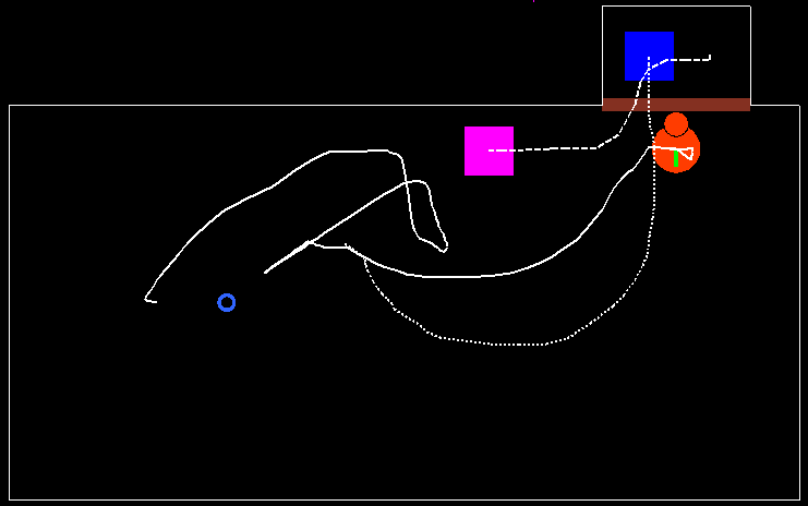
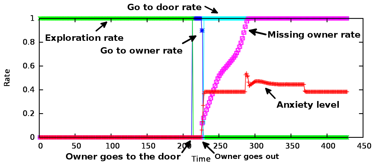
Fig. 68 shows the values of four state variables on a time scale (iteration number). Two immediate changes can be seen which are both caused by events related to the movement of the owner. First when the dog realizes that the owner is heading for the door (around the 200th iteration) the exploration rate drops rapidly and the rate of the ‘DogGoesToOwner’ behaviour component is high, till the owner finally leaves the room (around the 250th iteration). When the owner had left the room, the‘DogGoesToDoor’ behaviour component will be active, causing the value of the ‘Missing the owner’ state to increase. At the same time the anxiety level of the dog also increases with the leaving of the owner.

In the second example the ‘DogGoesToOwner’ behaviour will be presented in details from another point of view than the previous example. As its name suggests, this behaviour component is responsible for determining the need to go to the owner for the dog. The description of this behaviour component is more complex than the rule base in the previous example. The complete rule base for the ‘DogGoesToOwner’ behaviour is shown in REF _Ref364164389 \h , where the last column means the consequent part, all the other columns are antecedent dimensions (the ‘x’ value in the rule description means that the value of that antecedent is omitted while reasoning – does not have effect in the rule). The explanation of the terms used in the rule base is the following (‘observation’ in this case means that the value is gathered (measured) directly from the environment, ‘previous state’ means that the value was calculated in the previous iteration as a conclusion of a rule base):

dgtd – previous state – dog goes to door rate (zero-large) – see Fig. 6-12 for the corresponding fuzzy partition

dgto – previous state – dog goes to owner rate (zero-large) – see Fig. 6-12 for the corresponding fuzzy partition

oir – observation – owner is inside (true-false) – see Fig. 6-9 for the corresponding fuzzy partition

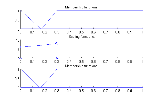
ddo – observation – distance between dog and owner (zero-large) – see Fig. 6-10 for the corresponding fuzzy partition

dgtt – previous state – dog goes to toy rate (zero-large) – see Fig. 6-9 for the corresponding fuzzy partition

dgro – previous state – dog greets owner rate (zero-large) – see Fig. 6-9 for the corresponding fuzzy partition

dpmo – previous state – dog’s playing mood rate with the owner (zero-large) – see Fig. 6-9 for the corresponding fuzzy partition

dpms – previous state – dog’s playing mood rate with the stranger (zero-large) – see Fig. 6-9 for the corresponding fuzzy partition

danl – previous state – dog’s anxiety level (zero-large) – see Fig. 6-11 for the corresponding fuzzy partition

ogo – observation – owner is going outside (true-false) – see Fig. 6-9 for the corresponding fuzzy partition

dgto (consequent) – next state – dog goes to owner rate (zero-large) (output)

The rules can be interpreted as the following textual description, in the corresponding order:

dog goes to door do not go to owner

dog should greet the owner go to owner

dog is nervous go to owner

dog's playing mood with owner is high go to owner

owner is going out of the room go to owner (follow the owner)

dog is calm and dog is not playing and not greeting do not go to owner

owner outside do not go to owner (can’t go to the owner)

dog is going to the toy do not go to owner

dog's playing mood with stranger is high do not go to owner

already going to owner and owner is near do not go to owner (arrived at the owner)

already going to owner and owner is far going to owner (keep on going)

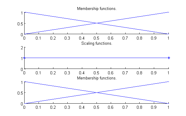
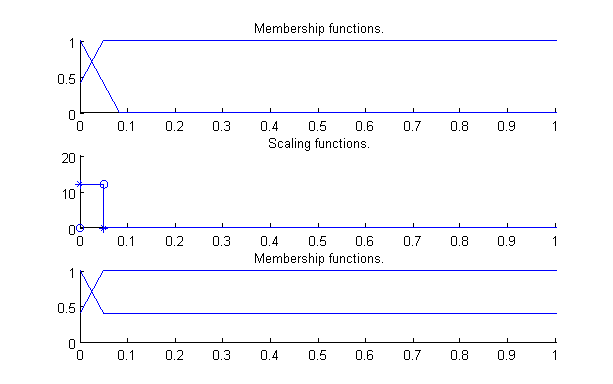
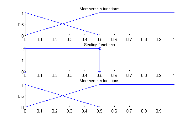
The presented rule base is suitable to define a complex behaviour component with only eleven rules in spite of the relatively high antecedent dimension count (ten variables) thanks to the usage of FRI. In Fig. 6-9 through Fig. 6-12 the fuzzy partitions used for the various antecedents are presented. From top to bottom the curves in the mentioned figures show the membership functions, the scaling functions REF _Ref385687747 \r \h and the reconstructed membership functions (based on the scaling function). As it can be seen most of the fuzzy partitions are simple (six of the nine antecedents use the same simple fuzzy partition), consisting of only two triangular fuzzy sets with their cores at 0 and 1, and steepness of 1 on the right and the left side respectively. This is true also for the other rule bases in the model, most of the antecedent variables are defined by fuzzy partitions exactly like the one shown in Fig. 6-9.

Most of the behaviour components defined in the system are responsible for coordinating the movement (heading direction) of the dog, which must be aggregated by some kind of behaviour fusion. The simulation uses a simple weighted sum of the currently required behaviour components for determining the movement vector of the agent. Other behaviour components can be executed in parallel with movement related components. Also there are rule bases which are responsible for calculating the rate of behaviour components which are not directly executed, but instead their values are used by other rule bases as input values (in a hierarchical manner). E.g. the ‘DogGreetsOwner’ component is not executed directly, as shown in REF _Ref364164389 \h \* MERGEFORMAT . the consequent of ‘DogGreetsOwner’ is used as an input value in the rule base of the ‘DogGoesToOwner’ behaviour component, hence the actual output behaviour will be triggered by the activation of the ‘DogGoesToOwner’ behaviour component.

The model can be customized for different types of dogs. The system provides three factors for customization (‘Parameters’ in Fig. 6-4), which can be set in the interval [0,1]: ‘Anxiety’, ‘Acceptance’, and ‘Attachment’. The ‘Anxiety’ parameter defines the level of anxiety of the dog on a scale between calm and nervous, ‘Acceptance’ defines the level of the dog’s acceptance towards the stranger (between friendly and unfriendly), ‘Attachment’ defines the level of attachment of the dog to its owner (between weak and strong attachment). In fact these parameters are not directly used in the behaviour description rule bases. Secondary variables are calculated first based on the three parameters. Then these secondary parameters are used in the corresponding fuzzy rule bases. The three external parameters (‘Anxiety’, ‘Attachment’, ‘Acceptance’) mentioned earlier are used as antecedents in various rule bases, which have the task of determining the values of secondary parameters. These secondary parameters are then directly used as antecedents in the rule bases of the fuzzy automaton driving the simulation. These calculated secondary parameters are the following:

Play without the owner (when the owner is outside)

Do not play with the stranger (even when it could be possible)

Run in circles (caused by anxiety) when stranger is inside

Run in circles (caused by anxiety) when the dog is alone

Base rate of greeting the stranger

Base rate of greeting the owner

Base rate of following the stranger, when he/she is leaving the room

Base rate of greeting the owner, when he/she is leaving the room

Base rate of stress (anxiety)

Base rate of standing at the door

Base rate of standing at the door, even when the owner is inside

Base rate of passivity

This hierarchical strategy is useful for minimizing the input dimensions of the rule bases (one input variable is used instead of three input values in this case), hence fewer rules are required. The values of the secondary parameters are also calculated using fuzzy rule interpolation, each secondary parameter having its own rule base for determining the exact value based on the three input parameters. These are calculated at the time of initialization before starting the simulation, but can be also adjusted while the simulation is running, allowing the operator to switch between different types of dogs in real-time.

A distinct, but important part of the framework is the so called observer module (see Fig. 6-4), which has the task of evaluating the model (the correctness of the constructed rule bases) itself. The observer module only gets information from the environment (just what an outsider would see), no data about the inner states of the fuzzy automaton or behaviour weights are supplied to the observer. Based on these observations the observer module is able to determine what kind of activity is going on in the simulation. It can distinguish among ‘playing’, ‘exploring’, ‘standing at door’ and ‘passive’ states. If the dog is in contact (close the human and looking at the human) with the owner or the stranger, that is also measured and logged. Furthermore a special scoring system developed by ethologists used for evaluating the separation and reunion episodes (human leaves dog / human comes back) is also implemented in the observer module. Also the overall time spent in the various states along the different episodes is measured. A summary of the measurements and the scores is calculated at the end of the simulation, which can be directly used by ethologist experts to evaluate the simulated dog in the same manner as they would with real dogs.