Digital Servo Drives
Copyright © 2014 Dr. Korondi Péter, Dr. Samu Krisztián, Raj Levente, Décsei-Paróczi Annamária, Dr. Fodor Dénes, Dr. Vásárhelyi József, Dr. Vass József

A tananyag a TÁMOP-4.1.2.A/1-11/1-2011-0042 azonosító számú „ Mechatronikai mérnök MSc tananyagfejlesztés ” projekt keretében készült. A tananyagfejlesztés az Európai Unió támogatásával és az Európai Szociális Alap társfinanszírozásával valósult meg.

Published by: BME MOGI
Editor by: BME MOGI
2014
- 1. Introduction
- 2. Classification of electric motors
- 3. Classification of electric drives
- 4. Sliding mode control
- 4.1. Short historical overview
- 4.2. Introductory example
- 4.3. Solution of differential equations with discontinuous right-hand sides
- 4.4. Control relays
- 4.5. The solution of the differential equation of the introductory example
- 4.6. Design of the sliding manifold is state-space approach
- 4.7. Discrete-time sliding mode design
- 4.8. Sliding mode Introductory example
- 4.8.1. Derivation of system trajectory
- 4.8.2. Error trajectory
- 4.8.3. Simple switching strategy
- 4.8.4. Explanation of sliding mode
- 4.8.5. Robustness of sliding mode control
- 4.8.6. Time function
- 4.8.7. Design of Sliding mode control
- 4.8.8. Comparison of sliding surface design methods
- 4.8.9. Control law
- 4.8.10. Switching surface of sliding mode
- 4.8.11. Observer based sliding mode
- 5. Internet based measurement of the servo motor
- 5.1. Aim of the measurement
- 5.2. Introduction
- 5.3. System overview
- 5.4. Presentation tools for measurement
- 5.5. General guidelines to experiments
- 5.6. Using the PCI-1720 D/A card – Motion control/ Exercise 1.
- 5.7. Using the real-time clock with PCI 1720 D/A card – Motion control/ Exercise 2.
- 5.8. Using the PCI-1784 Counter card – Motion control/ Exercise 3.
- 5.8.1. Initializing the PCI-1784 card by the function of DRV_DeviceOpen (see Exercise 1.)
- 5.8.2. Reset counter values on PCI-1784 card by the function: DRV_CounterReset
- 5.8.3. Start counting operation on PCI-1784 card by the function of DRV_CounterEventStart
- 5.8.4. Read counter values on PCI-1784 card by the function of DRV_CounterEventRead
- 5.8.5. Sample program of counter operations on PCI-1784 card
- 5.9. Open Loop Control measurement – Motion control/ Exercise 4.
- 5.10. Closed Loop Control Measurements – Motion control/ Exercise 5.
- 6. Sample measurement
- 6.1. Using the PCI-1720 D/A card -- Exercise 1
- 6.2. Using the real-time clock with PCI 1720 D/A card – Exercise 2
- 6.3. Using the PCI-1784 Counter card -- Exercise 3
- 6.4. Open Loop Control measurement – Motion control/Exercise 4. Open-loop test
- 6.5. Closed Loop Control Measurements -- Exercise 5
- 6.5.1. Parameter tuning of the P controller -- Test 1.
- 6.5.2. Step signal response of the P controller -- Test 2.
- 6.5.3. Response of the P controller to step changes in the reference speed signal -- Test 3.
- 6.5.4. Response of the P controller to step changes in the load -- Test 4.
- 6.5.5. Step signal response of the PI controller -- Test 2.
- 6.5.6. Response of the PI controller to step changes in the reference speed signal -- Test 3.
- 6.5.7. Response of the PI controller to step changes in the load -- Test 4.
- 6.5.8. Step signal response of the P and PI controller -- Test 1.
- 6.5.9. Stick-slip phenomenon
- 6.5.10. Step signal response of the position controller with inner shaft speed controller -- Test 1.
- 6.5.11. Fault tolerance measurements
- 6.5.12. Control of time-delay system
- 6.5.13. Sliding mode control results
- 6.6. Complex design and measurement
- 6.6.1. State feedback and its design
- 6.6.2. Application of reference signal correction
- 6.6.3. Design of the state observer
- 6.6.4. Integral control
- 6.6.5. Identification of the system
- 6.6.6. Design of the control
- 6.6.7. Identification of the motor
- 6.6.8. Design of the control
- 6.6.9. Integral control
- 6.6.10. Filter design for velocity measurement
- 6.6.11. Implementation
- 6.6.12. Control without integrator
- 6.6.13. Results of the measurement
- 6.6.14. Control with the integrator
- 6.6.15. Results of the measurement in the case of integrator
- 6.6.16. Appendix
- 7. Modelling Induction Motors
- 8. Sensorless Control with Speed Estimators
- 9. Glossary of SYMBOLS
- References
- 2.1. Movement types of electric motors
- 2.2. Intermediate medium of electric motors for energy transfer
- 2.3. Classic and inside out stator and rotor designs
- 2.4. Path of flux in electromagnetic motors
- 2.5. The directions of the magnetic momentums in four neighbouring domain caused by the loop currents originating from the spin of the electrons.
- 2.6. Torque types
- 2.7. Most commonly used motor names
- 2.8. Single-phase asynchronous motors
- 2.9. Reluctance motors
- 2.10. Permanent magnet motors
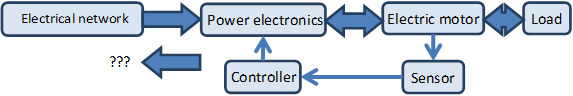
- 3.1. Main components of electrical drives
- 3.2. Simple DC drive
- 3.3. Simple AC drive
- 3.4. Interpretation of the four quadrants
- 3.5. Signs of the current and voltages in all four quadrants
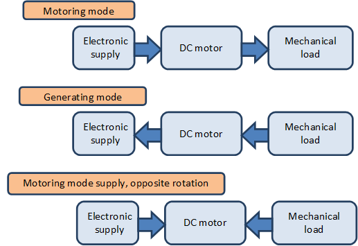
- 3.6. Direction of energy flow in different modes
- 3.7. AC drive using direct AC-AC converter
- 3.8. Usual layout of the servo drives
- 4.1. L-C circuit
- 4.2. Possible state-trajectories.
- 4.3. Removing the error.
- 4.4. Controller with relay
- 4.5. The state trajectory sliding along the surface S
- 4.6. The f(x) vector space pointing towards the surface S.
- 4.7. Introductory example
- 4.8. System trajectory
- 4.9. System trajectory
- 4.10. Error trajectory
- 4.11. Error trajectory
- 4.12. Simple switching strategy
- 4.13. Explanational animated figure about sliding mode control
- 4.14. Robustness
- 4.15. Time function
- 4.16. Design of Sliding mode control
- 4.17. Comparison
- 4.18. Control law
- 4.19. Switching surface
- 4.20. Observer based implementation
- 4.21. Application
- 4.22. Measurement results
- 5.1. System setup
- 5.2. Maxon A-max 26(110961) DC motor
- 5.3. Voltage change circuit diagram
- 5.4. Real circuit of voltage change
- 5.5. Maxon Planetary Gearhead GP 26(110395)
- 5.6. Maxon Digital Encoder HP HEDL 5540
- 5.7. Homepage layout
- 5.8. Exercise selection
- 5.9. Exercise results
- 5.10. Real-Time Extension architecture
- 5.11. Construction (http://dind.mogi.bme.hu/animation/chapter1/1.htm)
- 5.12. Equivalent circuit (http://dind.mogi.bme.hu/animation/chapter1/1_1.htm)
- 5.13. Time-domain equations (http://dind.mogi.bme.hu/animation/chapter2/2.htm)
- 5.14. Frequency-domain equations (http://dind.mogi.bme.hu/animation/chapter2/2_1.htm)
- 5.15. Derivation of transfer function of the DC motor (http://dind.mogi.bme.hu/animation/chapter2/2_2.htm)
- 5.16. Derivation of the time constants of the DC motor (http://dind.mogi.bme.hu/animation/chapter2/2_3.htm)
- 5.17. Derivation of state space representation (http://dind.mogi.bme.hu/animation/chapter3/3.htm)
- 5.18. Steady state, static characteristics (http://dind.mogi.bme.hu/animation/chapter3/3_1.htm)
- 5.19. Interactive figure of the static characteristics (http://dind.mogi.bme.hu/animation/chapter3/3_2.htm)
- 5.20. Analysis of the disturbance transfer function (http://dind.mogi.bme.hu/animation/chapter3/3_3.htm)
- 5.21. MatLab simulation of the motor
- 5.22. Analysis of the transfer function (http://dind.mogi.bme.hu/animation/chapter3/3_4.htm)
- 5.23. The MatLab model of the approximations
- 5.24. Bode diagram of a normal third order filter
- 5.25. Bode diagram of a third order Bessel filter
- 5.26. Classical PI controller (http://dind.mogi.bme.hu/animation/chapter4/4.htm)
- 5.27. Determination of the remaining phase margin (http://dind.mogi.bme.hu/animation/chapter4/4_1.htm)
- 5.28. Application (http://dind.mogi.bme.hu/animation/chapter4/4_2.htm)
- 5.29. Bode-diagram (http://dind.mogi.bme.hu/animation/chapter4/4_3.htm)
- 5.30. Note to classical PID controller (http://dind.mogi.bme.hu/animation/chapter4/4_4.htm)
- 5.31. Step response (http://dind.mogi.bme.hu/animation/chapter4/4_5.htm)
- 5.32. MatLab simulation of the controller motor
- 5.33. Position of the PI controller (http://dind.mogi.bme.hu/animation/chapter4/4_6.htm)
- 5.34. Response for load disturbance (http://dind.mogi.bme.hu/animation/chapter4/4_7.htm)
- 5.35. MatLab simulation of the speed control loop of the motor
- 5.36. Speed and current controller (http://dind.mogi.bme.hu/animation/chapter4/4_8.htm)
- 5.37. Explanation for neglecting the internal feedback line with kФ. (http://dind.mogi.bme.hu/animation/chapter4/4_9.htm)
- 5.38. Design concept (http://dind.mogi.bme.hu/animation/chapter4/4_10.htm)
- 5.39. Determination of Tu parameter (Tu ≈33 ms)
- 6.1. Sinusoidal output voltage
- 6.2. Open loop control Torque=1
- 6.3. Open loop control Torque=0.1
- 6.4. Comparison of unfiltered and filtered velocity
- 6.5. Comparison of different filters
- 6.6. Comparison of digital filters (period 0.1 s). Reference torque:l ight blue, unfiltered: blue, normal filter: green, Bessel filter: red
- 6.7. Comparison of digital filters (period 0.4 s). Reference torque: light blue, unfiltered: blue, normal filter: green, Bessel filter: red
- 6.8. P controller results for parameter tuning
- 6.9. P controller tuned by Ziegler Nichols method (P = 2.3)
- 6.10. P controller results for 3 step changes in the reference speed value
- 6.11. P controller results for step change in load
- 6.12. PI controller results for step change in the reference speed value
- 6.13. PI controller results for 3 step changes in the reference speed value
- 6.14. PI controller results for step change in load
- 6.15. P controller results for step change in the reference position
- 6.16. Stick-slip phenomenon
- 6.17. Position controller with P controller for position and PI inner shaft speed controller
- 6.18. Results of the position controller with P controller for position and PI inner shaft speed controller
- 6.19. PI control with a velocity filter
- 6.20. PI control with a velocity filter
- 6.21. PI control with a velocity filter
- 6.22. PI controller with and without anti windup function
- 6.23. Integral term without anti windup function
- 6.24. Integral term with anti windup function
- 6.25. Ultimate gain
- 6.26. PI controller for time delyed system
- 6.27. Reference signal correction in Discrete time
- 6.28. Observer based state feedback
- 6.29. Observer based state feedback with integrator
- 6.30. State feedback by integral control
- 6.31. Angular velocity with respect of time
- 6.32. Angular velocity with respect of time
- 6.33. Angular velocity with respect of the moment
- 6.34. Change of the angular velocity
- 6.35. Compare of the model and the measurement
- 6.36. The response of the step function
- 6.37. Model of the simulation
- 6.38. Results of the simulation
- 6.39. Moment
- 6.40. States
- 6.41. Model of the simulation with the integrator
- 6.42. Results of the simulation
- 6.43. Moment
- 6.44. Angular velocity
- 6.45. Step response
- 6.46. Bode diagram
- 6.47. Step response
- 6.48. Filtering
- 6.49. Result of the measurement
- 6.50. Results of the measurement in the case of integrator
- 7.1. An asynchronous motor
- 7.2. Classification of electric motors
- 7.3. Sinusoidal Current density distribution
- 7.4. Cross section of an Induction Motor
- 7.5. Three-phase stator and rotor windings of an asynchronous motor in the natural coordinate system
- 7.6. The coordinate systems for machine equation transformation
- 7.7. Equivalent circuit of the AC motor in normal operation
- 7.8. Equivalent circuit of fluxes
- 7.9. Vectorial diagram of fluxes and voltages
- 7.10. Modified equivalent circuit with the elimination of stator leakage
- 7.11. Modified equivalent circuit for fluxes if the rotor leakage is eliminated
- 7.12. Equivalent circuit of the motor valid also for transient operation
- 7.13. The chosen equivalent circuit
- 7.14. Connection between different coordinate systems
- 7.15. MATLAB/SIMULINK model of the AC motor
- 7.16. Maximal and Nominal Torque vs. Speed
- 7.17. Structure of a closed-loop scalar control with volts/hertz and slip regulation
- 7.18. The vector diagram of FOC principle
- 7.19. Basic scheme of FOC for AC-motor
- 7.20. Blockdiagram of a three Phases Asynchronous Motor Driver Using a FOC
- 7.21. Flux identification model in the case of a rotor-flux–oriented coordinate system
- 7.22. SIMULINK model of the rotor flux identification
- 7.23. FOC control of the induction motor
- 7.24. SIMULINK implementation of the FOC control block
- 7.25. The applied Torque
- 7.26. - components of the stator current
- 7.27. Rotor flux - components
- 7.28. The speed and reference speed in the case of FOC
- 7.29. d-q components of the stator current
- 8.1. Structure of the Speed estimator - Kalman Filter Techniques (KFT)
- 8.2. Structure of the MRAS
- 8.3. Speed adaptive Luenberger Observer
- 8.4. Speed Adaptive Extended Luenberger Observer
- 8.5. State Vector Reconstruction
- 8.6. Luenberger Observer Structure
- 8.7. The iterative algorithm of the KF
- 8.8. Flow chart of the KF
- 8.9. Structure of the Kalman Filter
- 8.10. Structure of the EKF
- 8.11. Off-Line identification
- 8.12. On-Line identification
- 8.13. Structure of the EKF based sensorless control
- 5.1. Parameters
- 5.2. Parameters
- 5.3. Parameters
- 5.4. Parameters
- 5.5. Parameters
- 5.6. Parameters
- 6.1. Ziegler-Nichols tuning chart
Chapter 1. Introduction
The aim of Digital Servo Drives study material is to give an overview of electrical motion devices used in mechatronic systems. The basic working principles and steady state operation of DC motors and asynchronous motors are considered known. The main goal of this note is to give a systematization of the existing knowledge.
Chapter 2. Classification of electric motors
In the chapter title the term electric motors was intentionally used instead of the commonly used electrical machines, because we would like to express that neither the transformers nor the generators used in power plants - both are parts of the topic electrical machines - will be discussed in this syllabus. Naturally the majority of the motors discussed here have got energy regeneration mode (acting as generators) which also can be used for braking and furthermore they can be used for energy recuperation to achieve better efficiency. Some of the motors like the ultrasonic motors however cannot be used for energy recovery. Several different methods existing for classify the electric motors. From the users’ point of view the main difference between electric motors is the movement type (i.e. linear or rotary). See Figure 2-1.
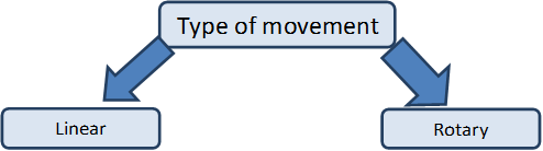
In theory all types of electric motors can produce linear and rotary movement it is only a question of construction of the motor. Most of the electric motors producing rotary movement thus in this syllabus only the rotary motors will be discussed.
The main question about the working principle of the different type of electric motors is which medium is used to relay the rotary movement from the motor’s stator to the rotor. (See Figure 2-2.)
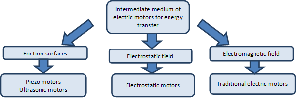
Negotiations about this question have only begun in the late 20th century. In the 20th century only the electromagnetic motors were considered as electric motors. Although the working principles of the electrostatic motors were known in the middle of the 18th century but electrostatic motors couldn’t produce significant amount of torque at that time and technological level, thus they were used to drive instruments rather than for energy conversion. Their importance has increased again in Micro Electro Mechanical Systems (MEMS), where as a general rule to be stated the inductors were replaced by capacitors. The electrostatic motor is a type of electric motor that operates on the basis of attraction and repulsion of the electric charge, thereby the coil is replaced by condenser. An important difference between the two motor types is that in case of the electromagnetic motors, the motor power varies approximately linearly with the volume, while the output power per unit volume may increase significantly when reducing the size of an electrostatic motor. The reason is that the maximum available magnetic flux density in the air gap inside the motor depends on the saturation of the ferromagnetic material used in the motor. In the electrostatic motors the maximum field strength is limited by the dielectric strength of air, whoever it is known, that the dielectric strength of the air at same values of the air’s physical properties (temperature, pressure, humidity) is increased for small electrode distances according to the Paschen’s law. Therefore, the integration of many small electrostatic motors can open up interesting perspectives. In robotics often mentioned problem is that if we compare the ratio of human muscle and total body weight ratio to the motors performing the motion of robots and robots’ full weight, then we can see that the drive mechanism is relatively too heavy for robots. One solution could be to replace the current motors ferromagnetic material. The so-called coreless motors were appeared as one trend of weight reduction, but in this context the so-called high-performance electrostatic motors are providing an alternative. At the time of writing this note the electrostatic motors are still in the experimental stage, despite this as an encouraging result a 100W electrostatic motor was appeared on the market, which weighs approx. an order of magnitude smaller than an electromagnetic motor weighs with similar nominal power.
The Piezo motors, also known as ultrasonic motors are forming the youngest generation of electric motors. Nowadays the Piezo motors almost became the dominant electric motors of the camera optics drive systems. Their advantage is the faster and more silent positioning on focus. A small disturbance can be caused by trademark reasons; the various manufacturers had to use different names.
Some trademarks and their manufacturers:
USM (UltraSonic Motor) (Canon);
SWM (Silent Wave Motor) (Nikon);
HSM (HyperSonic Motor) (Sigma);
SSM, (SuperSonic Motor) (Sony);
SDM (Supersonic Drive Motor) (Pentax);
SWD (Supersonic Wave Drive) (Olympus);
XSM, (Extra Silent Motor), (Panasonic);
USD (Ultrasonic Silent Drive) (Tamron).
In addition to the Photography industry the term most commonly used is USM. In the micro-and nanotechnology the Piezo actuators also have a particular role. Piezo motors should be used in places where no ferromagnetic materials can be used for some reasons for example in MRI devices a magnetic field with a magnitude of 9T may possible, in ferromagnetic materials a magnetic field with a magnitude of 2 T can also cause problems. But the use of electromagnetic motors is also not advisable in the vicinity of superconductors. Later on we briefly describe the electrostatic and the Piezo motors.
2.1. Electromagnetic motors
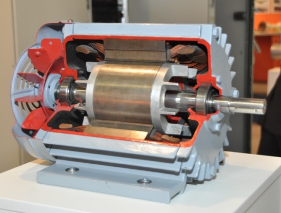
The rotary motors are consisting of a tubular section and a cylindrical section. The rotational movement is enabled with the use bearings. Generally, the tubular part is the stator fixed to the external environment, in which the cylindrical portion rotates, but the roles can mixed up, typically in the case of wheel hub motors and fans and including the so-called Coreless motors. (See Figure 2-3.)
The laws of electromagnetic machines:
The operation of electromagnetic machines is based on the interaction of two electric or magnetic fields which are at rest relative to each other.
The operation of electromagnetic machines is reversible i.e. the direction of the energy flow can be reversed.
Theoretically the efficiency of the electromagnetic machines can approximate the 100 % freely.
The most important step of operation of the electromagnetic motors is the creation of the magnetic field (excitation). The excitation can be inserted on the:
stator (one side excitation);
rotor (one side excitation);
both (two sides excitation).
The excitation can be accomplished by
winding;
permanent magnets.
The excitation must be varied relative to the stator or to the rotor. This can be achieved only if an external power source is used for the excitation of the windings. Thus always at least one of the stator-rotor excitations is achieved with windings, the other one can be a winding or a permanent magnet. This means that on every electromagnetic motor there is an actual winding, but in general sense all of these motors can be modelled with a stator winding and a rotor winding, which are in inductive interaction with each other.
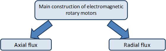
The magnetic field lines are always forming a closed curve. In terms of the magnetic field fundamentally two different types of the electromagnetic motors can be distinguished. See Figure 2-4.)
In the case of an exciter winding with a number of turns N the following can be written:
| (2.1) |

Where  is the exciting current,
  is the magnetic field strength, and
  is the closed curve of the magnetic flux’s path.
It is known that to describe the magnetic field two different physical quantities are used. One of them is the  magnetic induction that describes the total magnetic field. The other one is the
  magnetic field strength, which takes into account only the impact of the so-called external currents. The relationship between the two quantities:
| (2.2) |

Where  is the permeability of vacuum, and
  is the relative permeability. The foregoing provides a link between the two different approaches of magnetic field, the latter taking into account the effect of the material. Unpaired electrons (on a given the electron path, only one electron orbits, details should be found in the scope of quantum physics) in materials have a permanent magnetic moment, which can strengthen the effect of sending magnetic field. This can be modelled simply with an elementary loop current consequence of the electron’s orbital movement. This can be construed as the elementary loop currents formed inside the material are creating elementary magnetic fields as well. The neighbouring elementary magnetic fields can strengthen each other while they are trying to organize themselves in a parallel shape (well below of the Curie temperature). The reasons for this phenomenon are also lying in the scope of quantum physics. So-called domains are formed inside the material, in which the elementary magnetic moments are completely parallel, however the absence of an external magnetic field the magnetic orientation of each of the domains are random, thus the individual domains are impairing each other’s effect (the magnetic field lines can close inside the material) and only a small magnetic field can be measured from the outside.
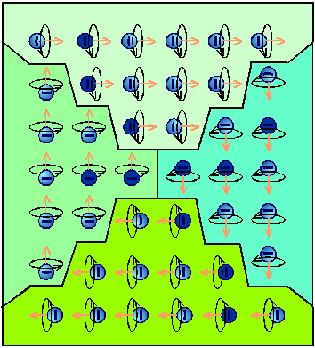
External magnetic field causes at first a shift of the boundaries of the domains so that it will strengthen the external magnetic field. The shift of boundaries has a nearly linear range where the total magnetic field varies nearly proportionally whit the external magnetic field, in which the domains are then rotated into the direction of the external magnetic field. When all of the domains were turned, than the material can no longer continue to strengthen the external magnetic field, this is called full saturation. In terms of torque generation the magnetic induction  is dominant. The goal is to achieve the maximum possible magnetic induction and minimize the required excitation. This is the reason that the electromagnetic motors are made of ferromagnetic material. In case of ferromagnetic materials at unsaturated state
 . This means that the same magnetic induction can be created and the scattered flux also can significantly be reduced if ferromagnetic material is used in the magnetic circuit and if the machine is designed so that the saturation cannot occur, than the excitation current can be reduced up to several orders of magnitude. Of course, there is an air gap between stator and rotor because of constructive reasons, but in terms of the magnetic circuit the goal is to the air gap should be as small as technologically possible. As we will later see, the spatial distribution of the air-gap flux density can be also an important design consideration, and therefore there are motors, where the size of the air gap is not constant, but for those motors is also true that the minimal air gap should be as small as possible.
2.1.1. Torque of electromagnetic motors
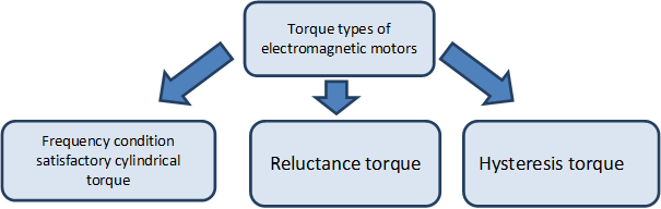
The unified theory of electrical machines distinguishes three kinds of steady-state (non-zero mid value) torque types. (See Figure 2-6.)
The first two torque types (similarly as the electromagnets’ pull force) can be calculated via the use of the so called principle of virtual work. According to this principle for the motor’s infinitely small  rotation at constant excitation will change the energy
  stored in the motor’s magnetic field. It is assumed that the magnetic field neither uses electric power from the electric circuitry nor gives unnecessary energy to it. According to the principle of energy conservation the change in the energy amount of the magnetic field equals to the change of the
  mechanical energy needed for the same rotation assuming
  rotor angular speed is constant.
| (2.3) |
In case of windings the energy of the magnetic field can be easily calculated as energy stored in an inductor. If the number of turns on the winding is noted as  the energy stored in an inductor:
| (2.4) |
Where if  than
than  is the self-induction factor, if
  than
than  the mutual inductance.
Because of symmetry reasons:
| (2.5) |

If the time is stopped at a particular moment, the current will have to be seen constant, and therefore the induced voltage is zero on the winding, i.e. the magnetic field really does not take up and does not give off energy from and to the electric circuit. The change in the energy of the magnetic field is derived solely from changes of the inductance. The inductance changes due to changes in the position of the rotor. Indicate the values of the frozen currents with  and
and  the torque in the particular moment:
| (2.6) |
Of course, if the time freezes at every moment one after another then the following can be written:
| (2.7) |
2.1.1.1. Cylindrical torque of Single-phase motor
The frequency condition is applies for motors with inductive connection, cylindrical interior design (with constant air gap) and the motors are modelled on both sides with coils, thus the corresponding torque is called cylindrical torque.
Assumptions:
single-phase windings can be found on both sides;
eddy currents aren’t formed on either side and the magnetizing curve of the iron core has no hysteresis;
the spatial distribution of the induction in the air gap generated by each coil is sinusoidal;
the principle of superposition is valid for the magnetic field (magnetization of ferromagnetic material is linear and non-saturated);
the function of each coil’s current is a sine wave (as a limiting case including the direct current and permanent magnetic excitation as well);
the supply currents on both sides are in the same phase;
the coils are symmetrical (the mutual inductance is a sinusoidal function of the rotor’s angular position with a period equal to the time needed for one rotation).
It is known, that
| (2.8) |
Where  and
and  are the self-induction factors in the stator and the rotor,
  is the mutual inductance in linear case,
  and
and  are the exciter currents in the stator and rotor respectively and
  is the rotor’s actual angular position. In (2.8) only the third part is a function of the rotor’s actual angular position and in case of constant angular velocity can be calculated as:
| (2.9) |
Where  is the load angle (the starting angular position of the rotor, depending on the load). Based on (2.3) and (2.8) substituting the sinusoidal currant and (2.9) we can get
| (2.10) |

Where  is the amplitude of the stator’s current,
  is the amplitude of the rotor’s current,
  is the maximum value of the mutual inductance between the stator and the rotor (in the angular position of
  ),
),  is the angular speed of the rotating magnetic field of the stator relative to the stator,
  is the angular speed of the rotating magnetic field of the rotor relative to the rotor,
  is the rotor’s angular speed relative to the stator. In general case (2.10) would produce a pulsating torque (with zero mid value). This fact has a strong relationship with another fact, that a single-phase coil can only produce a pulsating magnetic field. The frequency condition refers for those cases where (2.10) have a non-zero mid value. The first condition is the sinus value of the load angle shouldn’t be equal to zero.
| (2.11) |

Further conditions, which can’t be satisfied simultaneously (therefore a pulsating torque is always present in case of a single-phase motor)


2.1.1.2. Cylindrical torque of Multi-phase motors
In case of multi-phase motor windings of the stator and the rotor are modelled with two coils on both sides.
Assumptions:
eddy currents aren’t formed on either side and the magnetizing curve of the iron core has no hysteresis;
the two windings are perpendicular on each other on both sides;
the two pairs of the windings are geometrically completely symmetrical, (the values of the mutual inductances are changing in sinusoidal relationship with the rotor’s angular position, and the with has period equal to the time needed for one rotation);
the spatial distribution of the induction in the air gap generated by each coil is sinusoidal;
the principle of superposition is valid for the magnetic field (magnetization of ferromagnetic material is linear and non-saturated);
the function of each coil’s current is a sine wave (as a limiting case including the direct current and permanent magnetic excitation as well);
the currents supplying the motor are symmetrical on both sides, the amplitude of the feeding currents’ of the windings are equal on the same side;
The phase of the supplying currents is 90º (one of the supplying currents is sinusoidal the other one is cosinusoidal);
Starting phases of all of the currents are zero (purely sinusoidal or cosinusoidal).
In the two-phase winding system only the rotor’s angular position dependent component of the stored energy  is given, because all other parts are eliminated while making the partial derivatives.
| (2.16) |

| (2.17) |

Based on the assumptions for the feeding current and (2.9)
| (2.18) |

Utilizing the sinusoidal functions and the symmetry of the windings the equation of the torque can be simplified as were before using (2.18). This has a strong correlation with that the two-phase winding supplied by symmetric, but phase shifted current can generate rotating magnetic field.
| (2.19) |
The frequency condition is one of the single-phase cases.
| (2.20) |

If the (2.20) frequency condition is true than the torque is constant (no pulsating torque):
| (2.21) |
(2.20) is one frequency condition satisfying case.
DC current supplied DC motor
Constraint condition | Resulting condition | ||
|
| (2.22) |


The above means that because of the commutator the current of the rotor which seems from the exterior standing is actually rotating in the opposite direction of the rotor with the exact same angular speed compared to the rotor.
AC current supplied DC motor (let  be the angular frequency of the AC current)
Constraint condition | Resulting condition | ||
|
| (2.23) |


It can be seen that there is no theoretical obstacle for supplying a DC motor with AC current. This is the theoretical basis of the universal motors.
DC current supplied / permanent magnet rotor excited motor
Constraint condition | Resulting condition | ||
|
| (2.24) |


In these machines steady-state torque is only generated when the angular frequency of the AC current supplying the rotor, more specifically the angular speed of the magnetic field generated by the stator’s winding is equal to the angular speed of the rotor, this angular speed is called synchronous speed. Between the axis of the rotating magnetic field and the axis of the rotor is the  load angle. Thus follows if the synchronous machine is supplied directly from sinusoidal voltage network than synchronous machine has no starting torque. In contrast, if the synchronous speed is controlled by electronics than any speeds can be reached within the operating range. The condition for this is to know the angular position of the rotor (actual angular speed). This is the theoretical basis of the brushless motors.
Asynchronous (induction) motors
Constraint condition | Resulting condition | ||
|
| (2.25) |


There is no supply on the rotor of an asynchronous motor (an exception is the doubly fed asynchronous motor), thus by default the angular frequency of the induced voltage on the rotor is equal to the difference between the synchronous speed and the angular speed of the rotor (as a boundary situation at the synchronous speed the amplitude of the induced voltage is zero). In the above cases motors with DC current excitation on one side or AC current with identical frequency and phase excitation on both sides were explained (AC current supplied DC motor), therefore the last condition was irrelevant. In case of induction motor the last condition would only be satisfied if the winding on the rotor would be purely ohmic but in a real motor this never happens. It is clear without detailed explanation that in case of purely inductive winding on the rotor (with the rotation of currents in the winding of the rotor by 90º and subtracted back to (2.18)) the generated torque would have a zero middle value. If someone would like to produce the windings on the rotor from superconductors than the asynchronous motor wouldn’t have any torque output. In other words in case of asynchronous motor the simplified form of torque equation (2.19) should have a part, which takes in to account the impedance of the winding of the rotor with a cosine function of the phase angle, which has a maximum value at the zero phase
angle point (in case of pure ohmic impedance). The angular frequency – torque curve of the asynchronous motor can also be interpreted. At the synchronous speed the motor don’t generate any torque because the current of the rotor is zero. As the slip is increased so do increasing the induced voltage of the rotor, and thus the amplitude of the current is increasing as well. The ohmic resistance of the rotor winding independent from the slip (neglecting the skin effect), in contrast, the inductive reactance of the winding will increase as the slip is increasing, thus worsening the phase angle of the rotor current in terms of the maximum available torque. There are two opposite effects what are prevailing if the slip is increased, one of them is increasing the other one is decreasing the generated torque. In these cases there is always an optimal operating state, where the torque is at maximum, this is called pull-out torque. The deep groove and double squirrel cage motors are designed intentionally so that the skin effect may improve the phase of the rotor current at the start of the motor. Thus higher generated torque can be reached with less current consumption (details are known from the basics of asynchronous motors).
Remarks
There are no limits for the values of the currents in (2.20), but the linear magnetic behaviour condition of the materials should be provided, if the excitation is too large the magnetic material can reach saturation.
In most of the practical applications the supply is a voltage source, thus opposing the approach of the above calculations, the actual torque can’t be calculated from the known current but instead the actual load torque will determine the actual current consumed.
2.1.1.3. Reluctance torque
If the air gap height is not constant (typically when protruding poles can be found on the rotor), than on the other side (typically on the stator) the self-induction factor will became a function of the angular position of the rotor. Usually the reluctance and cylindrical torques are occurring combined, here the only case will be described where the stator is supplied and the rotor has protruding poles without excitation. Thus this means there are no eddy currents on the rotor, if eddy currents would develop on the rotor, than they should be considered as excitation and that will lead to a similar operating mode as the induction motors have. In case of soft iron core rotor the polarity is irrelevant, therefore the inductivity value is changing a period of two during one rotation of the rotor.
Assumptions:
one single-phase winding can be found on the stator;
eddy currents aren’t formed on either side and the magnetizing curve of the iron core has no hysteresis;
the principle of superposition is valid for the magnetic field (magnetization of ferromagnetic material is linear and non-saturated);
the protruding poles and the stator winding is symmetrical (the self-inductance is a sinusoidal function of the rotor’s angular position with a period double the time needed for one rotation);
the function of the coil’s current is a sine wave.
Single-phase case will be detailed here, momentary value of the energy stored in the stator winding:
| (2.26) |
where  is the angular position independent part and
  is the angular position dependent part of the stator self-induction coefficient. In (2.26) only the last part is angular position dependent, and assuming constant angular speed it can be described by (2.9). Based on (2.3) and on (2.26) and substituting the sinusoidal currents and (2.9)
| (2.27) |
Using trigonometric identities
| (2.28) |

Constant torque can be achieved based on the first part of (2.28) if
| (2.29) |

This means that the reluctance motor has starting and holding torque. Based in the second and third part of (2.28)
| (2.30) |

this means for reluctance motors the frequency condition can be satisfied only at the synchronous speed, but there is no preferred direction of rotation (the motor can be rotated in both directions at the same power supply). The load angle is multiplied by 2, which means the maximum torque is generated if . All of the above statements are in full accordance with our physical ideas of the reluctance motors.
Remarks
The single-phase reluctance motors always have pulsating torque component similarly to the single-phase cylindrical torque, but in multi-phase reluctance motors the pulsating torque component can be eliminated similarly to the multi -phase cylindrical torque.
There is a preferred rotational direction for multi-phase reluctance motors.
In general the AC motors are supplied with sinusoidal voltage and therefore within the meaning of Faraday's law of induction the flux is sinusoidal, but in this case because of the variable self-induction factor the current in the coil cannot be sinusoidal.
In case of real reluctance motors some extent of cylindrical torque is generated because of the eddy current developing on the rotor, but in some cases the rotor is intentionally excited, thus the cylindrical and reluctance torque should be summed.
2.1.1.4. Hysteresis torque
Hysteresis torque is mainly utilized in small and fractional-horsepower machines. These synchronous motors are excited with permanent magnet rotor in accordance to the (2.24) frequency condition, where in asynchronous mode the rotor is allowed to change its magnetization. The eddy currents of the motor are still neglected but due to the magnetic reversal of the rotor the hysteresis loss must be taken in to account and therefore (2.3) cannot be used directly.
Suppose that we create a rotating magnetic field with a multi-phase winding and the motor is stalled. Let  denote the energy needed for the magnetic reversal. Let
  denote the mechanical energy needed for the magnetic field rotated once. Based on conservation of energy
| (2.31) |

Assuming constant  torque
| (2.32) |
If the motor is allowed to rotate than the rotation angle needed for one hysteresis loop in not equal to  and the kinetic energy of the motor must be taken in to account also in the energy balance.
| (2.33) |
Continuing the calculations with power instead of energy and neglecting stator side losses the mains absorbed power is equal to  air-gap power.
| (2.34) |

Equation (2.34) even has the same form as the air-gap power equation of the asynchronous motors with a difference that the power of copper loss is replaced by the power of the hysteresis loss. Also here the mechanical power and the power of the hysteresis loss can be expressed with slip and air-gap power:

The power of the hysteresis loss is independent from the load unlike the power of copper loss, and is only dependent of the relative angular velocity between the rotor and stator i.e. dependent on the slip. Consequently the air-gap power is constant, but furthermore the torque of the hysteresis motor is constant in the asynchronous mode.
| (2.37) |
Based on (2.37) the pure hysteresis motor will spin up in asynchronous mode generating constant torque until it reaches the synchronous speed then staying at synchronous speed it will continue rotating as a synchronous motor with a load angle depending on the magnitude of the load. In reality eddy currents are also developing on the rotor which are also generating cylindrical torque that satisfies the (2.25) frequency condition.
2.1.1.5. The impact of electronic power supply to the torque
In the previous chapters the spatial and temporal sinusoid being of functions was an important condition. The former one can be ensure by a proper mechanical construction and the power supply does not have any impact, but the later one is depending only on the power supply. In case of electronically powered motors harmonics in the excitation and pulsating torque caused by them, furthermore heightened losses compared to pure sinusoid supply must be expected. In extreme cases an electronically powered asynchronous motor can be overloaded (overheated) even operated at nominal speed and load conditions. This also means that if an induction motor is supplied directly from the electrical network and next to the motor is a power electronics device with non-sinusoidal power supply is operated and therefore the device is distorting the voltage of the electrical network than pulsating torque caused by harmonics in the excitation and heightened losses must be expected as well. Application of different type of filters is advisable if power electronics are operated to prevent the so called EMC (Electromagnetic compatibility) problems. With the use of control electronics the synchronous speed can be gradually changed both to synchronous and asynchronous motors.
2.1.2. Field-oriented approach method
There is force acting on a current-carrying wire when placed in a magnetic field.
| (2.38) |

where the overbar denotes spatial vectors,  is the force,
  is the magnetic induction,
  is the direction vector of the current-carrying wire and
  is the magnitude of the torque generating current.
The cross product is maximal when the magnetic induction vector and the path of the current are perpendicular to each other. This can be achieved by mechanical construction when the magnetic field is radial and the winding is axially oriented or inversely.
Based on (2.38) in the air-gap the magnitude of the magnetic field is critical, i.e. the magnetic induction should be maximal where the current-carrying wire is located in space.
Goal:
the
 value of the magnetic induction should be tuned by the excitation to an optimal value from the iron core’s point of view (to the maximum possible value, but way below of the saturation);
in case of flux weakening the
 magnetic induction should be controlled by the excitation;
the torque should be controlled only by the
 torque generating current.
The above principle can be most easily achieved with externally excited DC motor, thus these motors were used in classical servo drives. Nowadays this principle can be achieved even with induction motors.
Steps:
voltage, current and speed of the motor are measured (speed is approximated in sensor less applications);
based on the measurements the differential equation of the motor is solved for the magnetic flux;
currents are transformed in to the synchronously rotating coordinate system, where that orientation of the synchronously rotating coordinate system is searched for where
 and
and  can be separated easily;
a controller is to be designed for
 and
and  in the synchronously rotating coordinate system;
the control signals are transformed back to the stationary coordinate system;
the control signals are routed to the stator using PWM (Pulse Width Modulation).
2.1.3. Types of electromagnetic motors
The largest selection is available from the rotary electromagnetic radial flux type motors. All types will be discussed in detail in a later chapter. Here an overview will be given with a summary of the most important motor types. See Figure 2-7.
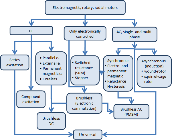 Figure 2.7. Most commonly used motor names
The DC and AC motors are the two most common motor types. The rotor of the former one is powered by DC voltage the stator if the later one is powered by sinusoidal voltage. The sinusoidal voltage can be single-phased but almost everywhere three-phase motors can be found if closed loop control is used. From the classification’s point of view it is an important property that in DC motors the magnetic field in the air-gap is trapezoidal, in AC motors it is sinusoidal.
DC motors can be further classified based on their excitation type. In the case series excited DC motors the rotor and the exciter winding which is developing the magnetic field are coupled in series together, in the case of parallel excitation they are coupled together in parallel. The supply of exciter winding can be independent from the rotor winding (this is called external excitation), or the exciter winding can be replaced by permanent magnet. Particular mention should be made for the coreless motors (these motors are available both in axial and radial flux type). Finally the so called compound or mixed excitation DC motors also exist. These motors have two exciter windings. One of the windings is coupled in series the other one is coupled in parallel. Particular mention should be made for the so called coreless motors, where this expression is valid only for the rotor more accurate name is coreless rotor motors. The rotor is assembled with epoxy based glue, thus no eddy currents are developing on the rotor and this is beneficial for the efficiency. One of their main advantages is the speed, because of the low moment of inertia of the rotor. The mechanical time constant can be in the millisecond order of magnitude, but typically such motors can be found only in the category of 100 W rated power or lower. The mechanical construction can be radial or axial flux type. For the radial type the rotor is cylindrical around the stator.
In case of classic AC motors the most important feature is the sinusoidal spatial distribution of the magnetic field in the air gap, which is sinusoidal in time also, because of the sinusoidal excitation voltage applied on the stator. If only one winding is excited then pulsating magnetic field will develop. The number of phases is also an important feature. If we want the magnetic field to have a rotating component, then two phase windings are needed spatially shifted around the circumference, which are supplied by time-shifted (phase shifted) voltage. Three phase windings are the optimal from many points of view. The non-industrial consumers (i.e. flats, offices) are supplied with single-phase power supply and therefore single-phase AC motors are required (for example older type washing machines, vacuum cleaners, or power tools). The importance of these machines is gradually decreasing, because the majority of motors are electronically supplied (even modern domestic machines) and with the use of power electronics any number of phases can be produced.
In case of three-phase AC motors the spatially- and time-shifted power supply will produce a rotating magnetic field and based on that the rotor will rotate together with the magnetic field or not in the motor mode operation we distinguish between synchronous and asynchronous motors. In case of classic (supplied by three-phase sinusoidal voltage) synchronous motors an asynchronous phase is required to be able to start the motor and reach the synchronous speed. The asynchronous motors are also called as induction motors. The rotor of asynchronous motors may contain actual winding and the terminals of the winding are slip rings. Thus these motors are also called slip ring motors. The rotor winding can be replaced by a short circuited cage thus these motors are called short circuited or squirrel cage motors. The synchronous rotation between the rotating magnetic field and the rotor can be reached if an electro- or permanent magnet is placed on the rotor. Further types of synchronous motors are the hysteresis and reluctance motors. The so called universal motors can be found mainly in power tools, which can be supplied with both AC and DC current. In theory the series excited DC motors can be supplied with AC current also. The difference between universal motors and series excited DC motors is that the rotor of universal motors is plated to minimize the core loss.
In this lecture note the single-phase motors won’t be discussed (in servo drive applications they are not used). For the classification of motors be complete in Figure 2-8. the most important single-phase motors are collected. Rotating magnetic field cannot be produced with single-phase winding only pulsating. In a stationary (not rotating), short-circuited winding will not develop torque if placed in a pulsating magnetic field, in other words the pure single-phase motor does not have starting torque. Conversely if the winding is rotating already in a pulsating magnetic field, then the torque will develop. The starting of the single-phase motor is critical. For this we can use partially shaded-pole, or split-phase, i.e. spatially shifted winding which is supplied through a capacitor and the capacitor will make the phase (time) shifting. The starting capacitor is only active when starting the motor and will be switched of once the motor is rotating. The run capacitor is always active, or we can use starting and run capacitors in combination. The universal motor is also a kind of single-phase motors.
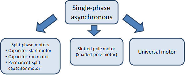 Figure 2.8. Single-phase asynchronous motors
The classical DC and AC motors can be operated without control electronics but if closed loop control is required than use of electronics is essential. There are motors however which cannot be operated without electronics. These motors are considered as synchronous machines (noted with arrows in Figure), but from these motors the classical synchronous motor specific asynchronous mode is missing, instead they can be accelerated or decelerated with the continuous change of the synchronous speed with the use of the electronics adapting to the speed of the rotor. This means also that instead of using asynchronous winding the rotor should be equipped with angular position sensor. Nowadays the so called sensor less drive is fashionable, where the angular position and angular speed of the rotor is approximated using mathematical calculations. The ordinary classification of electronically operated motors (AC and DC) can be confusing, and therefore was kept as a separate type. Including the stepper motors, switched reluctance motors and the brushless motors, which can be classified based on the shape of the magnetic field in the air gap. If the magnetic field in the air gap similarly to the DC motors is trapezoid, then the usual appellation is brushless DC motor (BLDC). If the magnetic field in the air gap similarly to the AC motors sinusoidal, then the usual appellation is brushless AC motor (BLAC). The PMSM is also a commonly used name; it is the abbreviation of the permanent magnet synchronous motor. The name on its own does not give information whether or not these motors are electronically operated, but usually only the electronically operated motors are considered as PMSMs. The brushless motors are also called electronically commutated (EC) motors.
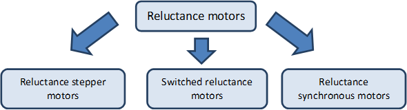
The Figure 2-7. is structured vertically but a number of horizontal correlations can be highlighted. In several motor types it is important for the torque generation that winding less (no excitation) protruding poles can be found on the rotor (the generated torque can be further increased if the poles are excited). These motors are called reluctance (magnetic resistance) motors. The name indicates that the magnetic resistance in the air gap is not constant. ???
Figure 29. summarizes the different types of reluctance motors. Basically the reluctance motors should be regarded as synchronous motors. The reluctance synchronous motors are supplied with three-phase sinusoidal voltage if operated without electronics, and there are windings on the rotor which are operated asynchronously thus taking care of the spin up of the motor. In case of switched reluctance motors the actual angular position of the rotor determines the excited windings on the stator. It follows that we must measure the actual angular position of the rotor. The switched reluctance motors are the most simplest by construction, there is no winding rotor on the Figure 2-9. .
In case of reluctance stepper motors the rotor will take an orientation according to the excitation of stator winding.
The permanent magnet is a fundamental component in many motor types. See Figure 210.
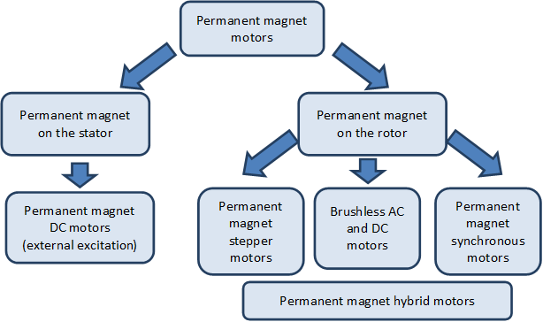
In comparison to the Figure new subclasses are the stepper motors with permanent magnet rotor and the hybrid motors. The hybrid name means the combination of permanent magnetic and non-permanent magnetic materials in the rotor. These motors are used in electric powered cars where the so called flux weakening technique is needed in order to reach higher angular velocities. The flux weakening is analogous to the mechanical torque converters used in motor vehicles, where if the angular speed is increasing so decreases the generated torque. In the low power (10 W) motors permanent magnet is used since long time ago, but for the appearance of the several kW brushless motors the spread of the rare earth magnets was a requirement.
2.2. Electrostatic motors
As the technology supporting our life of future, such as an energy problem and an aging society with fewer children, development of a hybrid car, an electric vehicle, and the robot that supports care and a life of people is furthered. And in order to develop these products, the motor which it is Small and Easy to treat and High efficiency and High power is indispensable.
The electromagnetic motor which has spread most now has a tendency which weight increases and efficiency drops with a higher power. These are the big problems as a future car or a robot's motor.
SHINSEI Corporation has till now offered the ultrasonic motor as an effective motor in the nonmagnetic environment, such as MRI which are medical facilities, superconductivity experiment equipment, etc.
The High Power Electrostatic Motor developed this time is a new style motor constituted by the technology in which ultrasonic motors completely differ. The High Power Electrostatic Motor (following ESM65-TR1) made as a trial production model is very lightweight compared with the electromagnetic motor of the same power. And on ESM65-TR1, since there is almost neither a friction part nor an exothermic part, energy efficiency is more than 95%. Moreover, ESM65-TR1 can show high performance in a vacuum environment. Furthermore, ESM65-TR1 can also be used in a nonmagnetic environment like an ultrasonic motor.
Chapter 3. Classification of electric drives
The difficulty of the classification of electric drives is caused by the fact that the drive systems are dedicated to specific motor types. Here an overview is given about the trends of the electrical drive systems based on some fundamental features. One classification point of view is how many motors (axles) are operated from one device. There are one and multiple axle electronic drives. In this lecture note only the one axle drives are explained. The main components of an electrical drive system can be seen in Figure 3-1.
The thick arrows denoting the way of energy flow. Depending on the actual application there may be a two-way energy flow at the load side. Electromagnetic motors are also capable of the two-way energy flow, but for the power electronic devices this is not always possible especially for the older types.
In the power electronics there are four different converter types can be distinguished:
DC-DC converter (DC chopper);
DC-AC converter (inverter);
AC-DC converter (rectifier);
AC-AC converter (AC choppers, thyristor-based cycloconverters, transistor matrix converters).
3.1. Simple drives
The power is usually supplied from the AC electrical network and therefore only the last two types of converters (AC-DC and AC-AC) would be enough. An example for that can be found in lower quality drives, which are using thyristors (or just a few transistors) (see Figure 3-2. and Figure 3-3.). In Figure 3-2. the one way arrows are symbolizing the mostly (not always) one-way energy flow. In case of AC motors because of the reactive power developing in the windings even in motor mode the two-way energy flow is required.


Primarily for DC drives it is an important classification point of view that in which quadrant (see Figure 3-4.) of the rotational speed-torque plain can the electrical drive operate the DC motor.

The four quadrants are determined by the direction of the supply voltage and current. Supposing an external excited DC motor let  be the armature voltage,
  be the armature current and
  be the induced voltage of the armature winding. The signs of the current and voltages in the quadrants of Figure 3-4. can be seen in Figure 3-5.
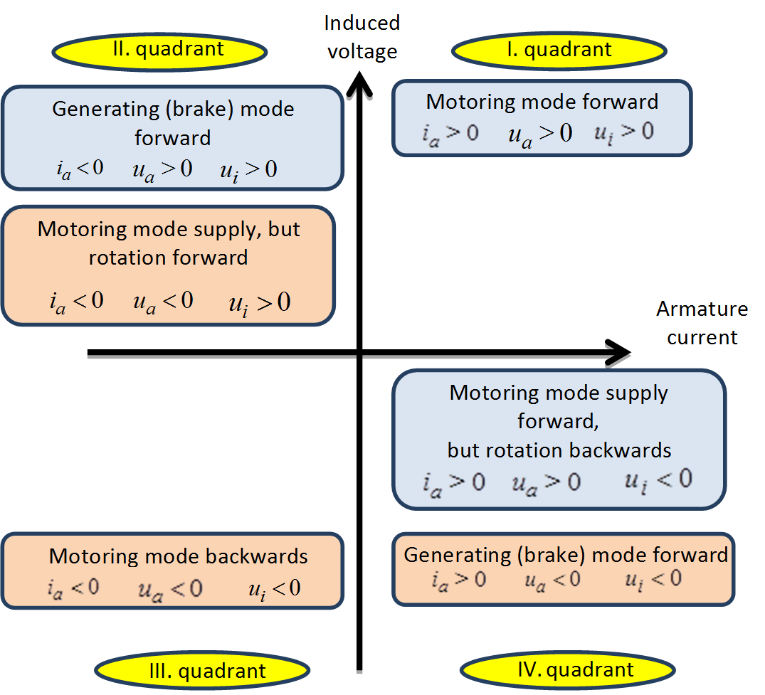
In motoring mode the directions of the voltage and the current are the same, the motor is consuming power from the electrical network (electric energy is converted to mechanical energy). The motoring mode needed for the rotating the motor forward and backwards can be found in the I. and III. quadrants. If for some reason the direction of the current changes then in any case the sign of the generated torque will also change. If the directions of the voltage and the current are the opposite of each other, then the electrical network will take up power (mechanical energy is converted to electric energy). This is called generating (brake) mode and can be realized in the II. and IV. quadrants. It is important to note that a DC motor can enter in the II. and IV. quadrants such a way that the directions of the voltage and the current are remaining the same (motoring mode), but the direction of motor rotation is changed via an external constraint. The asynchronous motors are also capable of this mode, but the synchronous motors are not. In the II. and IV. quadrants Mechanical energy is converted to electric energy in any case, however in case of the directions of the voltage and the current are the same then the motor will consume power from the electrical network as well. In other words both the electric and mechanical energy will be converted to heat; this means a negative impact for the efficiency of the drive. Resistor should be inserted into the electrical circuit of the rotor outside of the motor, on which the generated heat can be dissipated and to limit the current of the motor (in case of asynchronous AC and DC motors). This mode was necessary in case of a crane or elevator when the load is lowered in the past; because there were no cheap electronics available with generating mode at any rotational speeds. The generating mode can be achieved only at higher speeds than the no-load speed (in case of asynchronous motors above the synchronous speed) in case of DC supplied motor. Electronic control is needed for the manipulation of the supply voltage. In four-quarter servo drives the lowering of weights is done in generating mode regardless of the motor type. The generating mode is ensured by the electronics.
The directions of energy flow in the three different modes can be seen in Figure 3-6.
The rotational speed of an asynchronous motor supplied trough an AC chopper can be changed in a very limited extent. These systems won’t be discussed in this lecture note.
3.2. Four quadrants servo drives
First of all is noted that even for demanding AC drives direct AC-AC converters can be used (see ???
Figure 3-7. ), instead of using AC chopper the transistor matrix converter should be used (thyristor-based cycloconverters aren’t used nowadays). This solution isn’t adopted by the industry, but it can happen that this solution will prove industrially optimal.

Most of the servo drives are operated in all four quadrants and the conversion is done in two steps. First the mains voltage is rectified so will form an internal DC circuit, then with the use of a DC chopper in case of DC motor or with an inverter with changeable frequency in case of AC motor the given motor will be supplied. See in???
Figure 3-8. .
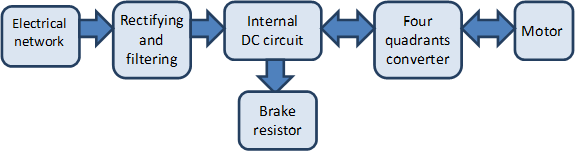
In Figure 3-8. there is only a one way arrow pointing outward from the electrical network box because nowadays this is typical. The most common and cheapest rectifiers are based on diodes and these units cannot feed the energy back into the electrical network. The brake resistor is used for dissipating the energy fed back from the motor. In case of diode-based rectifier the non-sinusoidal power supply means a more significant problem than the one-way energy flow, because these devices are taking up non-sinusoidal current and causing pollution to the electrical network. In many cases the diode-based rectifier is kept in the system but an electrical filter is inserted between the electrical network and the rectifier to minimize the electrical pollution. The sinusoidal current consumption can be achieved with open loop controlled rectifier. These devices are enabling the two-way energy flow and also acting as filters. This solution is not common nowadays, but in the near future it is possible for the industry to adopt the technology.
Only of the voltage or the current can be forced to the motor the other one will develop as a result, thus there are voltage and current source power supplies. The voltage source supply is easier to realize, but the current source supply has more direct relationship with the torque (see chapter 2.1.1), thus making the direct torque control more simpler. In the eighties and nineties were actual industrial applications using the so called current-source inverter (CSI) drive topologies. Nowadays the voltage-source inverter (VSI) drive topologies are dominant. This has technological reasons, but no one knows in which direction the technology will further develop in the future. Also in the eighties and nineties the so called resonant converters and in connection the so called soft-switching have appeared.
Most of the motors can be operated in four-quadrant mode.
The torque of synchronous motors can be positive and negative in both rotating directions, and extends into two quarters. In the former case the motor is in motoring mode, in the latter case the motor is in generating mode. The external excited DC motor and the asynchronous motor can enter in three quadrants at same voltage directions. In motor mode the rotational direction can change itself.
3.2.1. Torque sensing and measurement
In most cases the torque is not measured directly, but it is calculated from other electric parameters. The simplest and most inaccurate method for torque estimation is that the consumed power from the electrical network is calculated from the  voltage and
  current in the internal DC circuit.
| (3.1) |
This method is used in case of DC motors and asynchronous motors also. Especially for the asynchronous drives it is more complex and expensive using a more accurate direct method, which is based on measuring the actual current and voltage of the motor.
Chapter 4. Sliding mode control
- 4.1. Short historical overview
- 4.2. Introductory example
- 4.3. Solution of differential equations with discontinuous right-hand sides
- 4.4. Control relays
- 4.5. The solution of the differential equation of the introductory example
- 4.6. Design of the sliding manifold is state-space approach
- 4.7. Discrete-time sliding mode design
- 4.8. Sliding mode Introductory example
- 4.8.1. Derivation of system trajectory
- 4.8.2. Error trajectory
- 4.8.3. Simple switching strategy
- 4.8.4. Explanation of sliding mode
- 4.8.5. Robustness of sliding mode control
- 4.8.6. Time function
- 4.8.7. Design of Sliding mode control
- 4.8.8. Comparison of sliding surface design methods
- 4.8.9. Control law
- 4.8.10. Switching surface of sliding mode
- 4.8.11. Observer based sliding mode
4.1. Short historical overview
The sliding mode control has a unique place in control theories. First, the exact mathematical treatment represents numerous interesting challenges for the mathematicians. Secondly, in many cases it can be relatively easy to apply without a deeper understanding of its strong mathematical background and is therefore widely used in engineering practice. This article is intended to constitute a bridge between the exact mathematical description and the engineering applications. After a short overview of the sliding mode control the article presents its mathematical foundations, namely the theory of differential equations with discontinuous right-hand sides. The power electronic circuits, which always have some kind of switching elements, can be typically described by such differential equation. Such equations don’t fulfill the regular theorem of existence and uniqueness, but under certain conditions remain valid, if we interpret the solution of the differential equation according to the definition proposed by Filippov. The article presents a practical example of the definition proposed by Filippov per a sliding mode control of an L-C circuit and an experimental application on uninterruptible power supply.
Recently most of the controlled systems are driven by electricity as it is one of the cleanest and easiest (with smallest time constant) to change (controllable) energy source. The conversion of electrical energy is solved by power electronics. One of the most characteristic common features of the power electronic devices is the switching mode. We can switch on and off the semiconductor elements of the power electronic devices in order to reduce losses because if the voltage or current of the switching element is nearly zero, then the loss is also near to zero. Thus, the power electronic devices belong typically to the group of variable structure systems (VSS). The variable structure systems have some interesting characteristics in control theory. A VSS might also be asymptotically stable if all the elements of the VSS are unstable itself. Another important feature that a VSS - with appropriate controller - may get in a state in which the dynamics of the system can be described by a differential equation with lower degree of freedom than the original one. In this state the system is theoretically completely independent of changing certain parameters and of the effects of certain external disturbances (e.g. non-linear load). This state is called sliding mode and the control based on this is called sliding mode control which has a very important role in the control of power electronic devices.
The theory of variable structure system and sliding mode has been developed decades ago in the Soviet Union. The theory was mainly developed by Vadim I. Utkin [1] and David K. Young [2]. According to the theory sliding mode control should be robust, but experiments show that it has serious limitations. The main problem by applying the sliding mode is the high frequency oscillation around the sliding surface, the so-called chattering, which strongly reduces the control performance. Only few could implement in practice the robust behavior predicted by the theory. Many have concluded that the presence of chattering makes sliding mode control a good theory game, which is not applicable in practice. In the next period the researchers invested most of their energy in chattering free applications, developing numerous solutions.
After the introduction, the second section summarizes the mathematical foundations of sliding mode control based on the theory of the differential equations with discontinuous right-hand sides, explaining how it might be applied for control relay. The third section shows how to apply the mathematical foundations on a practical example.
4.2. Introductory example
The first example introduces a problem that can often be found in the engineering practice. Assume that there is a serial L-C circuit with ideal elements, which can be shorted, or can be connected to the battery voltage by a transistor switch (see Figure 4-1., where the details of the transistor switch are not shown). Assume that our reference signal has a significantly lower frequency than the switching frequency of the controller. Thus we can take the reference signal as constant.
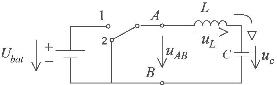
Assume that we start from an energy free state, and our goal is to load the capacitor to the half of the battery voltage by switching the transistor. The differential equations for the circuit elements are:
| (4.1) |


Due to the serial connection ic = iL, thus the differential equation describing the system is:
| (4.2) |
Introduce relative units such way, that LC = 1 and Ubat = 1. Introduce the error signal voltage ue = Ur - uc, where Ur = 1/2 is the reference voltage of the capacitor. Thus, the differential equation of the error signal has the form:
| (4.3) |


It is easy to see that the state belonging to the solution of (4.3) equation moves always clockwise along a circle on the phase plane  (see Figure 4-2.).
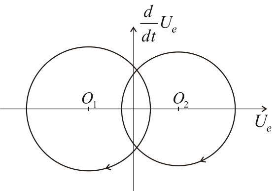
The center of the circle depends on the state of the transistor. The state-trajectory is continuous, so the radius of the circle depends on in what state the system is at the moment of the last switching. Assume that we start from the state
| (4.4) |
and our goal is to reach by appropriate switching the state
| (4.5) |
Introduce the following switching strategy:
| (4.6) |

where
(4.7) |
This means that if the state-trajectory is over the s = 0 line, then we have to switch the circle centered at O1, if it is below the line, then we have to switch the circle centered at O2. Examine how we can remove the error. Consider Figure 4-3., according to (4.6) and (4.7)(4.4) at first we start over the s = 0 line on a circle centered at O1. Reaching the line we switch to the circle centered at O2 so that the state-trajectory remains continuous. After the second switching we experience an interesting phenomenon. As the state trajectory starts along the circle centered at O1, it returns immediately into the area, where the circle centered at the O2 has to be switched, but the state-trajectory can not stay on this circle either, new switching is needed. For the sake of representation, the state-trajectory in Figure 4-3.reaches significantly over to the areas on both sides of the s = 0 line. In ideal case the state trajectory follows the s = 0 line on a curve broken in each points consisting of infinitely short sections switched by infinitely high frequency. In other words, the trajectory of the error signal slides along the s = 0 line and therefore is called sliding mode.
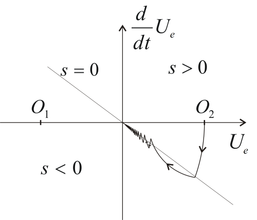
Based on the engineering and geometric approach we feel that after the second switching, the behavior of the error signal can be described by the following differential equation instead of the second order (4.3):
| (4.8) |

This is particularly interesting because (4.8) does not include any parameter of the original system, but the  we have given. Thus we got a robust control that by certain conditions is insensitive to certain disturbances and parameter changes. Without attempting to be comprehensive investigate the possible effects of changing some attributes and parameters of the system. If we substitute the ideal lossless elements by real lossy elements, then the state-trajectory instead of a circle moves along a spiral with decreasing radius. If the battery voltage fluctuates, the center of the circle wanders. Both changes affect the section before the sliding mode and modifies the sustainability conditions of the sliding mode, but in either case, the sliding mode may persist (the state trajectory can not leave the switch line), and if it persists, then these changes will not affect the behavior of the sliding mode of the system.
The next section will discuss how we can prove our conjecture mathematically.
4.3. Solution of differential equations with discontinuous right-hand sides
Consider the following autonomous differential equation system:
| (4.9) |

where
| (4.10) |

If f(x) is continuous then we can write (4.5) as the integral equation:
(4.11) |
The approach of (4.9) according to (4.11) is called Carathéodory solution, which under certain conditions may also exist when f(x) is discontinuous . Recently, several articles and PhD theses dealt with it how to ease the preconditions which guarantee the existence of (4.11) concerning f(x), but for the introduced example none of the cases might be applied, we need a completely different solution.
Filippov recommends a solution, which is perhaps closer to the engineering approach described in the previous section [3] [4]. Filippov is searching the solution of (4.9) at a given point based on how the derivative behaves in the neighborhood of the given point, allowing even that the behavior of the derivative may completely different from its neighborhood on a zero set, and regarding the solution ignores the derivative on this set. Filippov’s original definition concerns non-autonomous differential equations, but this article deals only with autonomous differential equations.
Consider (4.9) and assume that f(x) is defined almost everywhere on an open subset of  . Assume also that f(x) is measurable, locally bounded and discontinuous. Define the set K(x) for x
  f(x) by:
| (4.12) |
where  denotes the open hull with center x and the radius , is the Lebesgue measure, N is the Lebesgue null set and the word "conv" denotes the convex closure of the given set.
Filippov introduced the following definition to solve the discontinuous differential equation systems:
Definition:
An absolutely continuous vector-valued function  is the solution of (4.9) if
| (4.13) |

for almost every  . Note that if f(x) is continuous, then set K(x) has a single element for every x, namely f(x), thus the definition of Filippov is consistent with the usual differential equations (with continuous right-hand side). However, if f(x) is not continuous, then this definition allows us searching a solution for (4.9) in such a domain of x, where f(x) is not defined.
.
4.4. Control relays
Apply the definition of Filippov as a generalization of the introductory example in the case of such a controller with state feedback, where in the feedback loop only a relay can be found (see ???
Figure 4-4.). Assume that the state of the system can be described by the differential equation (4.9), where the vectorfunction f(x) is standing on the right-hand side rapidly varies depending on the state of the relay. The control (switching) strategy should be the following. In the domain of the space  defined by the fedback state variables define an n-1 dimensional smooth regular hypersurface S (which can also be called as switching surface) using continuous
  scalar-vector function in the following way:
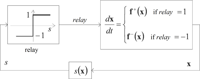
| (4.14) |
The goal of the controller is to force the state-trajectory to this surface. Mark the points of the surface S with xs. With the help of this surface we can divide the domain G into two parts:
Let the differential equation for x on domain G and our switching strategy have the following form:
| (4.17) |
where f +(x) and f -(x) are uniformly continuous vector-vector functions.
Note that f(x) is not defined on the surface S, and we did not specify that f +(x) and f -(x) must be equal on both sides of the surface S.
Outside the surface S we have to deal with an ordinary differential equation. Solution of (4.17) might be a problem in the xs(t) points of the surface S. According to definition (4.13), K is the smallest closed convex set, which you get in the following way: let’s take an arbitrary  hull of all xs(t) points of the xs belonging to the surface S, exclude f(xs), where f(x) is not defined (remark: it is a null set N domain), and we complete the set of f(x) vectors belonging to the resulting set to a closed convex set. Obviously, the smaller the value of
  , the smaller the resulting closed convex set. Finally, we need to take the intersection of the closed convex sets in the hull of all
  and N. Since f(x) is absolutely continuous, the following limits exist at any point of the surface S:
| (4.18) |
It means that the  set belonging to any point xs(t) of the surface S has only two elements, f +(xs) and f -(xs). We have to take the convex closure of these two vectors, which will be the smallest subset belonging to all
  values. In summary, the differential equation (4.9) with a (4.14) form discontinuity in the xs(t) points of S surface according to definition (4.13) can be described in the following form:
| (4.19) |
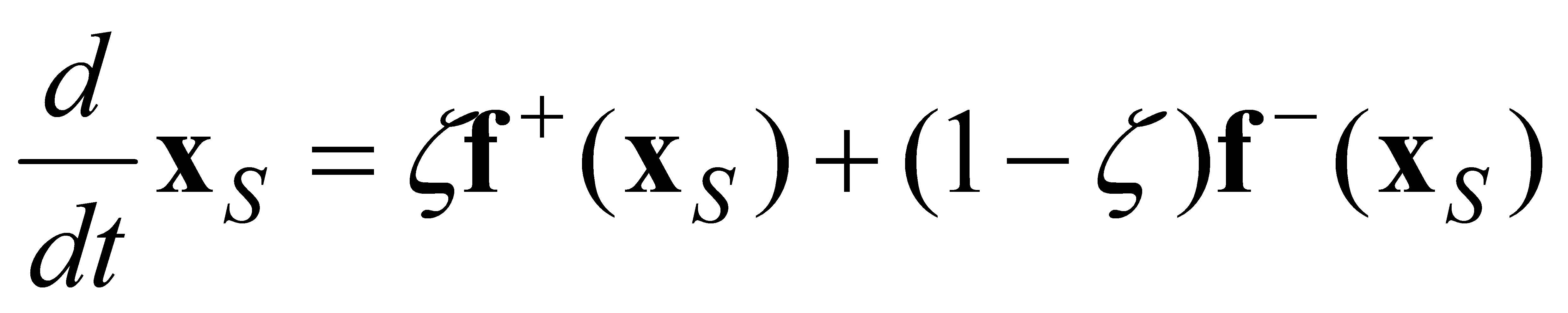
To illustrate (4.19) see ???
Figure 4-5., where we drew f +(xSP) and f -(xSP) vectors belonging to the point P of surface S. We marked the normal vector belonging to the point P of the surface with np. The change of the state trajectory in point xSP is given by the equivalent vector feq(xSP), which is the convex sum of vectors f +(xSP) and f -(xSP).
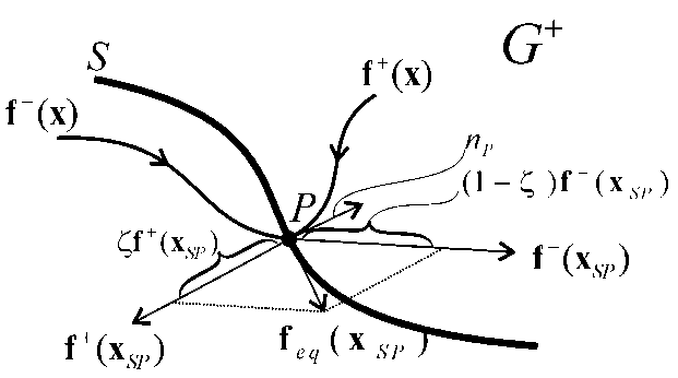
Denote by Lfs(x) the directional derivative of the scalar function s(x) concerning the vector space f(x):
| (4.20) |
where (a ● b) denotes the scalar product of vectors a and b. Since s(x) is uniformly continuous, the following limits exist at any point of the surface S:
| (4.21) |
The value of should be defined such that  and feq(xS) are orthogonal to the normal vector of the surface S (see Filippov 3. Lemma [3]):
| (4.22) |
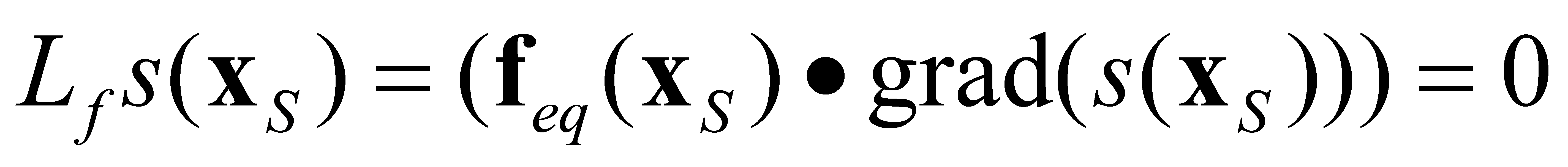
The equation (4.22) can be interpreted in the following way: in sliding mode, in the xs points of the sliding surface the change of the state trajectory can be described by an equivalent feq(xS) vector function that satisfies condition(4.22). Based on (4.19) and (4.22), we obtain
| (4.23) |
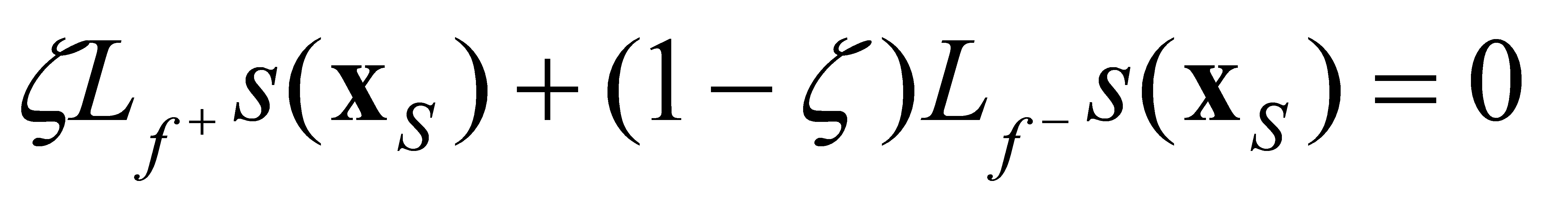
From (4.23) can be expressed:
| (4.24) |
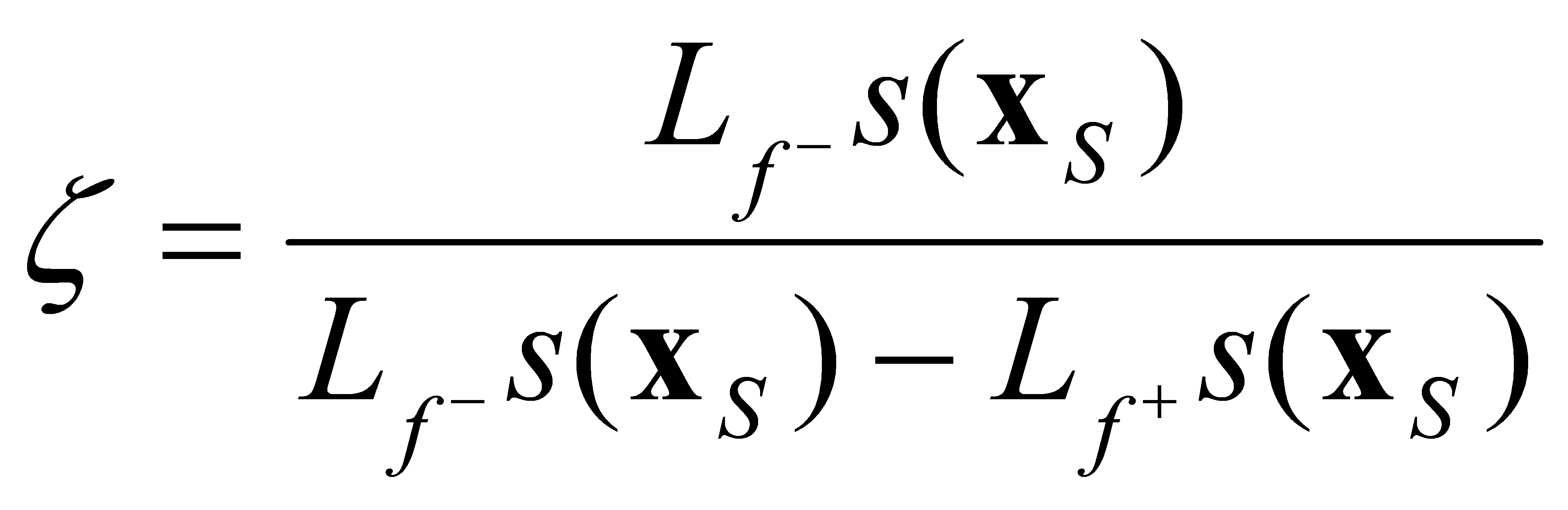
4.4.1. Condition for the existence of Sliding Mode
If  and
and  then on both sides of the surface S the vector space f(x) points towards the surface S (see Figure 4-6.). Therefore, if the state trajectory once reaches the surface S, it can not leave it. The state trajectory slides along the surface and therefore this state is called sliding mode.
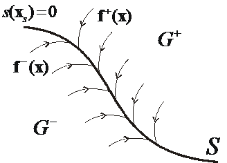
Note that the two conditions separately defined on both sides of the surface S:
can be substituted by one inequality:
| (4.27) |
Which can be interpreted as Lyapunov's stability criterion concerning whether the system remains on the surface S.
4.5. The solution of the differential equation of the introductory example
There are two energy storage elements (L and C) in the circuit of the introductory example, therefore the behavior of the circuit can be described by two state variables. The goal is to remove the voltage error, so it is practical to choose the error signal and the first time derivative of it as the state variables.
| (4.28) |
The state equation of the error signal, assuming that the reference signal Ur is constant:
| (4.29) |
where a22 = 0, if we neglect the losses assuming ideal L-C elements, while a22 = -R/L, if we model the losses of the circuit with serial resistance. Based on (4.6) and (4.7), let the scalar function defining, the sliding surface be:
| (4.30) |
Rewriting the matrix equation (4.29) to the form (4.17), we obtain:
| (4.31) |
where


The directional derivative of the scalar function s(x) concerning the vector space f(x) on both sides of the surface S is:

Note that in our case f +(x) and f -(x) can be defined on the surface S, therefore we do not need to calculate the limits in (4.21), the points  belonging to the surface S can be directly substituted. At the same time, (4.27) is met only in the following domain:
| (4.37) |
It means that, by the given control relay, only on a limited part of the surface S can be in sliding mode. By completing the relay control laws with additional members, we can reach that the condition of sliding mode is fulfilled on the whole S surface [5] [6]. In case of the control relay, based on (4.24) and (4.35), we get:
| (4.38) |
Based on (4.17), (4.31), (4.35), and (4.38) the differential equation describing the system in sliding mode will be:
| (4.39) |
The differential equation (4.39) is basically the same as the equation of the sliding line, and thus we can describe the original system as a first order differential equation instead of a second order one:
| (4.40) |
This way we proved, that the state belonging to the smooth regular sliding line S can be accurately followed by a state trajectory broken in each points consisting of infinitely short sections switched by infinitely high frequency. The solution of (4.40) is:
| (4.41) |

where Ues0 is the ues error signal at the moment when the state trajectory reaches the surface S. Based on (4.41) we can see that  is the characteristic time constant of the sliding line. Note that equation (4.41) does not include any parameter of the original system. This means that in the above-described ideal sliding mode the relay control law leads to a robust controller, insensitive to certain parameters and disturbances. The above derivation is only concerned with how the system behaves on the sliding surface, but we did not deal with the practically very important question of how to ensure that the state trajectory always reaches the sliding surface and stays on it.
Of course, in reality such an ideal sliding mode does not exist. From engineering point of view the challenge is the realization of a so-called chattering-free approximation of it.
4.6. Design of the sliding manifold is state-space approach
The following linear time invariant (LTI) system is considered; first the reference signal is supposed to be constant and zero.
| (4.42) |


| (4.43) |


The system (4.42) can be transformed to a regular form:
| (4.44) |
where
The switching surfaces of the sliding mode, where the control vector components have discontinuities, can be written in the following form:
| (4.45) |


When sliding mode occurs, σ = x2 + Kx1 and x2 = -Kx1. The design problem of the sliding surfaces can be regarded as a linear state feedback control design for the following subsystem:
| (4.46) |
In (4.46) equation, x2 can be considered as the input of the subsystem. A state feedback controller x2 = = -Kx1 for this subsystem gives the switching surface of the whole VSS controller. In sliding mode
| (4.47) |
Various linear control design methods based on state feedback are applicable to the design of the switching surfaces.
4.6.1. Linear Quadratic approach
According to LQ design the cost function (4.48) is minimized by solving the well known Riccati equation to achieve the optimal feedback gain for subsystem (4.46):
| (4.48) |
where ts (can be assumed zero) is the time at which sliding mode begins. (For simplicity, N = 0 is assumed.)
The LQ optimal sliding surface is given by
| (4.49) |


where P > 0 is a unique solution of the following Riccati equation:
| (4.50) |
4.6.2. Frequency shaped LQ approach
The frequency shaped sliding mode comes from frequency shaped LQ method. Frequency shaped LQ approach is based on frequency dependent weights. The cost function (4.48) can be written in the frequency domain using Perseval's theorem as
| (4.51) |
In the time domain (4.48), Q and R are constant matrices. If instead of a constant R, a frequency dependent weight matrix R(ω2) is introduced, control inputs for certain frequencies can be amplified or suppressed.
| (4.52) |
We can choose R to have high-pass characteristics for reduction of high frequency control inputs of the subsystem (4.46).
This idea is realized using state space representation. The frequency dependent weight R(ω2) must be a rational function of ω2 to solve this problem. The transfer function matrix W2(s) is defined as
| (4.53) |
where W2(s)* stands for the conjugate transpose of W2(s). The subsystem (4.46) should be augmented by the states (written in the vector xw2) of W2(s). W2(s) has the following state space representation
| (4.54) |
Then the cost function (4.52) with a frequency dependent weight matrix R(ω2) can be rewritten in the time domain as
| (4.55) |
where

Minimization of this cost function with cross term between state and control input is formulated as solving the following Riccati equation:
| (4.58) |

The optimal switching plane is written using the solution of this Riccati equation as
| (4.59) |

4.6.3. H∞ optimal control approach
Recently, linear control theory is well developed especially in the field of robust control. H∞ optimal control theory is an excellent result of this development. Hashimoto introduces H∞ control methods for the optimal sliding surface design based on H∞ norm.
The control goal is formulated through a norm minimization of the generalized plant G(jω), where H∞ norms are used to formulate the cost function. If G(jω) is a stable transfer matrix in the frequency domain, than the H∞ norms are
| (4.60) |
4.7. Discrete-time sliding mode design
Another kind of chattering is caused by the limited switching frequency of the control input. The robustness of continuous-time sliding mode control is obtained by high frequency switching of high-gain control inputs. To adapt the sliding-mode philosophy for a digital controller, the sampling frequency should be increased compared to other types of control method. To solve this problem asymptotic reaching of the sliding manifold has been proposed in literatures to avoid commutation. In an alternative idea, the samples of the system states belong to the sliding manifold after a finite number of sample steps.
Definition:
In the discrete-time dynamic system


a discrete-time sliding mode takes place on the subset of a manifold  if there exists an open neighborhood U of this subset such that from
  it follows
  .
.
According to this definition, the observer equation should be discretized at each sampling instant.
| (4.63) |
where subscript k means the k-th sampling time, i.e., t = kTs (Ts is the sampling period) and
| (4.64) |

The sliding surface should be discretized as well:
| (4.65) |


It follows from the definition that
| (4.66) |

for any  . The discrete-time sliding mode exists if matrix
  is invertible and control Uk is designed to satisfy (4.46):
| (4.67) |

By analogy with continuous-time systems, the solution of (4.67) is referred to as “equivalent control”.
| (4.68) |
The control law is chosen as follows:
| (4.69) |

where  is the physical limit of control signal
  .
.
This type of discrete-time sliding mode control law involves prediction. Knowledge of the model is necessary.
4.8. Sliding mode Introductory example
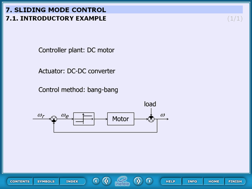
This static slide contains the basic idea of the sliding mode control. The controller plant is a DC motor, the actuator is a DC-DC converter and the control method is bang-bang.
This means that the DC motor is controller by a 2 state kind of relay which can accelerate or decelerate the motor. This control can switch when the system approaches the reference position but this causes big overshoot therefore the switching process must be occurred a little bit before that time. The question is: when. The next some slides give us the answer.
4.8.1. Derivation of system trajectory
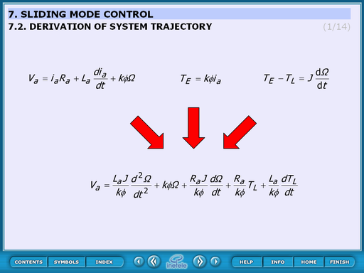
The bases of the transfer function are these equations:
| (4.70) |
| (4.71) |

| (4.72) |
And the transfer function:
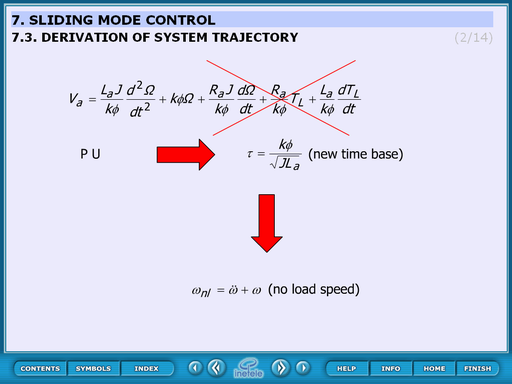
The basic of this derivation is the transfer function:
| (4.73) |
where the 3rd, 4th and the 5th member can be neglected (red cross shows the neglecting):
| (4.74) |
herefore:
| (4.75) |
Introducing the “per unit”:
| (4.76) |

The non-load speed:
| (4.77) |

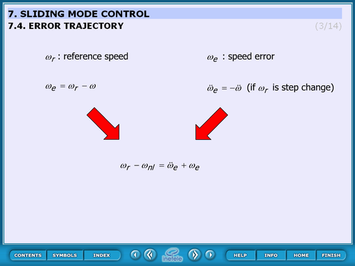
This slide derives the error trajectory.

– reference speed
| (4.78) |


– speed error
| (4.79) |

if  is the step change
| (4.80) |
4.8.2. Error trajectory
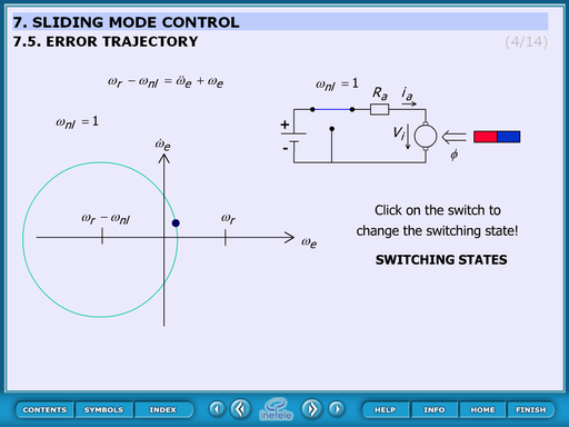
This animated figure displays the error trajectory when the switch is on or off.
Theoretical background:
The motor can be considered as a second order storage element which responds to the step change with oscillation. This oscillation appears as a circle in the ( ;
; ) diagram. The centre of the circle is
  when the switch is on (
 ) and
) and  when the switch is off (
 ).
).
Operation:
At start-up the switch is on and by clicking the switch it can be toggled between on and off state.
4.8.3. Simple switching strategy
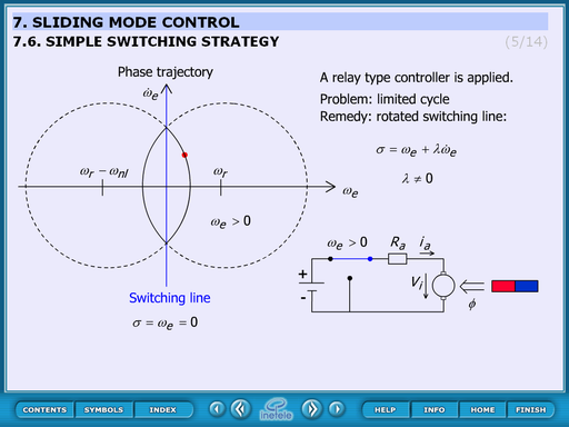
This animation sows the problem in case of the simplest control strategy. The process: the controller accelerates the motor until it reaches the reference speed. At this moment it switches and decelerates. But the system stores a lot of energy therefore overshoots. At the end of the overshoot the speed is higher than the reference and the system starts really slowing. But reaching again the reference speed and switching on the system would not accelerate immediately because of the storage capability. This process repeats and oscillation occurs.


The switching line is horizontal. To solve the oscillation problem the switching line should be rotated.
The animation cannot be controller actually. In the future built in buttons can be implemented is required.
4.8.4. Explanation of sliding mode
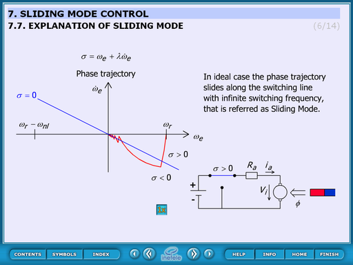
This animated figure explains the effect of the rotated switching line.
The trajectory slides from  in the direction of the switching line. When reaches the centre of the circle changes and the curve again to the direction of the sw. line.
The control of the animation:
It starts automatically and at the end it can be restarted by pressing ![]() button.
button.
This animation uses previously drawn figure. There is the possibility of changing this to function.
4.8.5. Robustness of sliding mode control
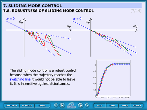
This static figure explains the robustness of the sliding mode control.
Theoretical background:
Once the control reaches the switching line the system becomes insensitive against disturbances because it won’t be able to leave the line. The way in which it reaches the line is independent from the result.
4.8.6. Time function
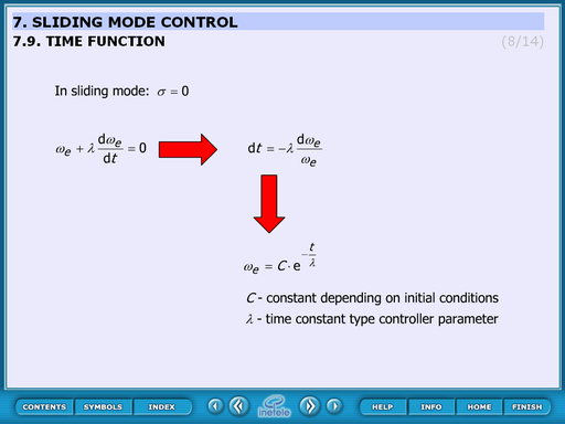
This animated slide derives the time function. Equations:
In sliding mode:
| (4.84) |

| (4.85) |

| (4.86) |

| (4.87) |

Where:
C – constant depends on initial conditions
- time constant type controller parameter
4.8.7. Design of Sliding mode control
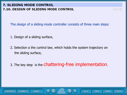
This slide concludes the screens until now. The text of the slide:
The design of a sliding-mode controller consists of three main steps:1. Design of a sliding surface, 2. Selection a the control law, which holds the system trajectory on the sliding surface,3. The key step is the chattering-free implementation.
4.8.8. Comparison of sliding surface design methods
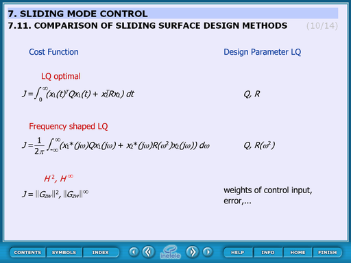
4.8.9. Control law
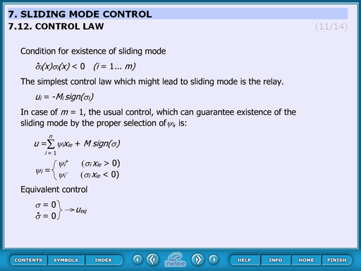
4.8.10. Switching surface of sliding mode
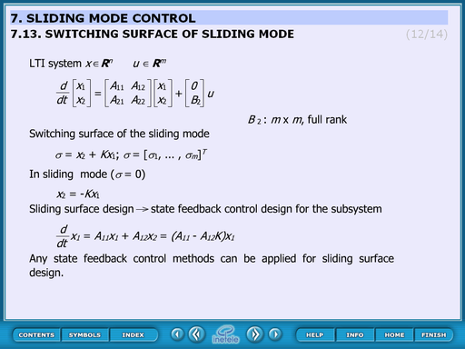
4.8.11. Observer based sliding mode
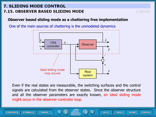
Application of sliding mode control
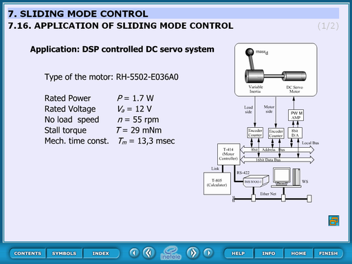
Measurement results of sliding mode control.
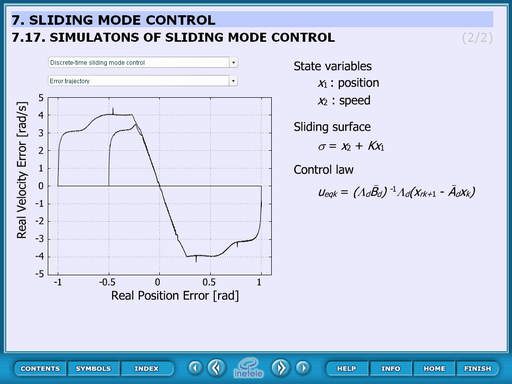
Chapter 5. Internet based measurement of the servo motor
- 5.1. Aim of the measurement
- 5.2. Introduction
- 5.3. System overview
- 5.4. Presentation tools for measurement
- 5.5. General guidelines to experiments
- 5.6. Using the PCI-1720 D/A card – Motion control/ Exercise 1.
- 5.7. Using the real-time clock with PCI 1720 D/A card – Motion control/ Exercise 2.
- 5.8. Using the PCI-1784 Counter card – Motion control/ Exercise 3.
- 5.8.1. Initializing the PCI-1784 card by the function of DRV_DeviceOpen (see Exercise 1.)
- 5.8.2. Reset counter values on PCI-1784 card by the function: DRV_CounterReset
- 5.8.3. Start counting operation on PCI-1784 card by the function of DRV_CounterEventStart
- 5.8.4. Read counter values on PCI-1784 card by the function of DRV_CounterEventRead
- 5.8.5. Sample program of counter operations on PCI-1784 card
- 5.9. Open Loop Control measurement – Motion control/ Exercise 4.
- 5.10. Closed Loop Control Measurements – Motion control/ Exercise 5.
5.1. Aim of the measurement
The user can learn from this measurement the control of a servo drive and robot by a computer. First the user gets acquainted with the communication between the computer and the servo drive as the important component of a mobile robot. Next, the embedded system of a mobile robot is studied (There is a separate Manual for robot experiment).
We will use a Digital-Analogue converter to send information from the computer to the servo drive since the reference signals are analogue voltage signals in most servos drives. The movement of the motor is measured by an encoder, which sends impulse train to the computer. A counter counts the impulses of the encoder and the computer can read the value of the encoder informing it on the position of the motor. The speed of the motor is calculated from the actual and the previous position information. This method results in a very noisy speed signal. The measurement uses a Discrete time filter to reduce this measurement noise. The user can learn the way of writing and tuning the PI controller for this simple servo drive.
The user does not need to be expert in computer programming, but she/he has to know the basics. The user will write some very simple program in C language and Visual Basic. Examples are shown and it is believed that the user can carry out this measurement even if it will be her/his first C or visual basic program.
The experiments are accessible on the following website:http://dind.mogi.bme.hu/experiment/
5.2. Introduction
To meet the competitiveness and environmental challenges in the manufacturing industry, automation and robotization is one of the most important trends i.e. turning the manual work power from tiring repetitive tasks into complex tasks where knowledge and human skills are required. This is both due to the increasing complexity level of products and the focus on improved working environment within EU. However, advanced robotic systems require advanced knowledge within many classical fields of engineering and surely in the small and medium size enterprises (SME), where all of these areas of expertises probably missing from the knowledge of the employees. Turning now to the problems of the advanced courses offered by universities, one of them is the different backgrounds of the attendees. In case of an advanced motion control course, one solution can be that the professor can refer to the internet for the necessary background. In this note new technology and new learning methods are combined. The interactive multimedia applications (animations, simulations, remote tasks) combined with the Web-based laboratory tests result in a Personal Learning Environment available all day around and all year around.
The DC motors have a special historical role in the field of industrial electronics since all industrial servo drives used DC motors in the past and the first microprocessor controlled drive [1] also applied DC motor. Even if they have several drawbacks they are used in recent applications [2] , [6] The main advantage of a DC servo motor drive is that it is simple from the point of view of control. Before the advent of micro controllers they were the only solutions for servo drive systems. It is easy to adopt various control methods for a DC servo system. It explains why some of the newly proposed control methods are frequently applied first for a DC servo system. On the other hand, there is a trend to control all kind of servo drives (field oriented induction motor drives [7] and brushless drives [8]) like a DC servo drive. PID controller is still the most common controller method in the industrial applications [9]. The other popular method is the sliding mode control that was introduced in the late 1970’s [10] but it is used recently in high-performance motion control systems [11]. In recent applications, the sliding mode control is combined with different soft computing methods [12], [13]. Sliding mode control of variable structure systems has a special role in the field of robust control. On one hand, the exact description of sliding mode needs advanced mathematics, which was established by [3], [4] in the early sixties. On the other hand, it is quite easy to implement in most engineering systems, only simple relay is necessary in most cases. To use the manual and perform the exercises the reader does not need to be familiar with most of the references listed.
5.3. System overview
Web based experiments play an important role in next generation of laboratories. The experiments can be operated around the clock. Access is provided whenever it is needed after booking. This manual deals with the control of DC servo motor and all necessary theoretical and experimental knowledge is included or referred to.
Following the manual’s instructions the users will acquire experience in PC based control of electrical systems, and in this specific case, in DC servo drive (Figure 5-1.).
In order to control the DC motor connected to PC, the following system components performing basic functions are needed:
A card generating analogue output signals to turn on/off the drive and generate the reference signal (e.g. D/A card).
A card receiving input encoder signal forwarding it to the PC (e.g. A/D card or counter card).
A real-time clock that can schedule signal sampling or task execution.
The users will start learning from the basics of programming of above mentioned cards through implementing modern control theories in real circumstances.
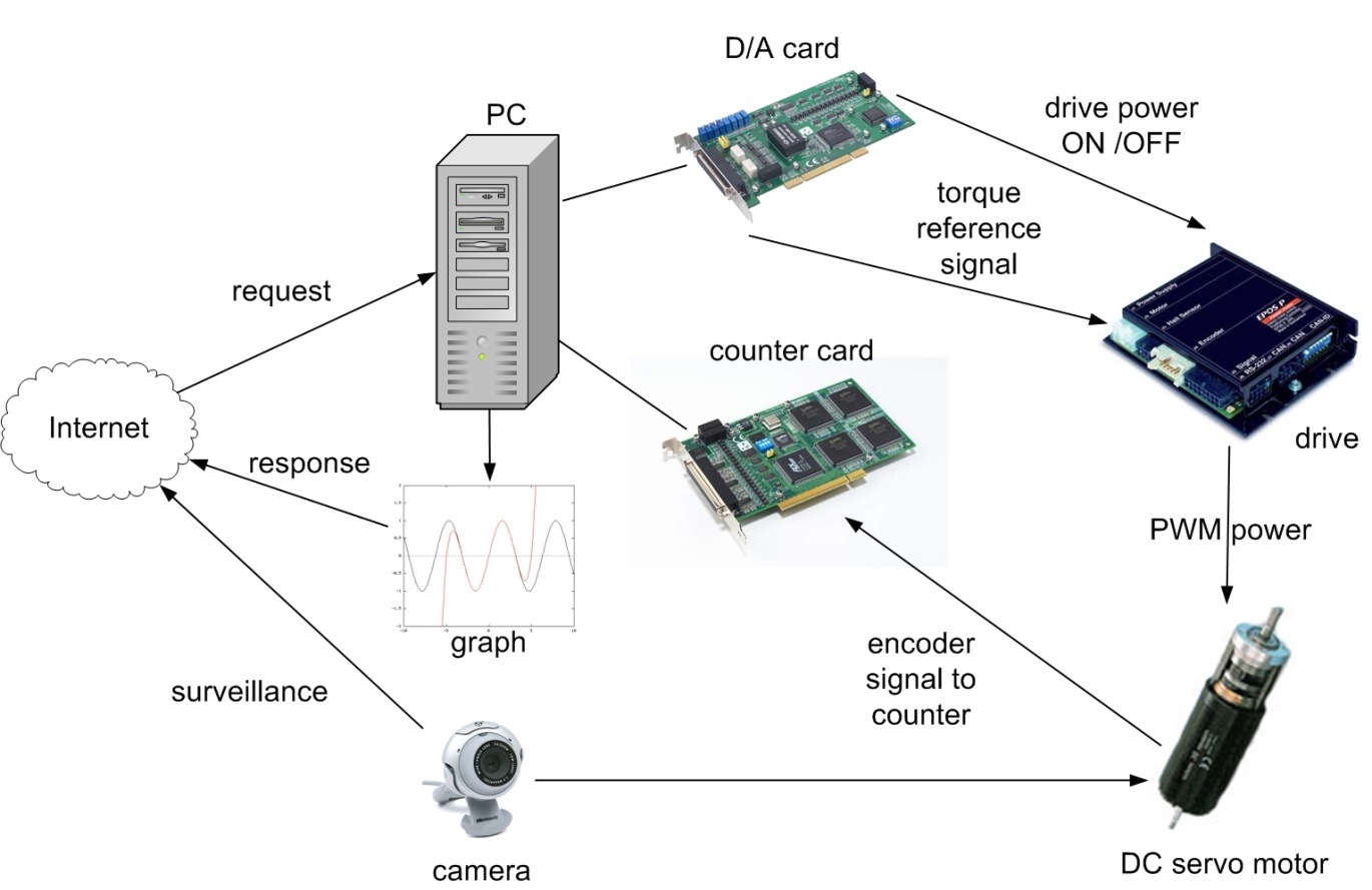
The key system components applied here are the following:
Industrial Siemens PC with Pentium 4, 2.8 GHz processor.
Advantec PCI-1720 D/A output card performing function 1.
Advantec PCI-1784 counter input card performing function 2.
Servo drive including:
Servoamplifier;
Maxon A-max 26(110961) DC motor;
Maxon Digital Encoder HP HEDL 5540;
Maxon Planetary Gearhead GP 26(110395).
WebCam for visualising the laboratory setup on the monitor.
MATLAB program.
The experiments are accessible on the following website:http://dind.mogi.bme.hu/experiment/
5.4. Presentation tools for measurement
Motor data from Maxon motor homepage: http://test.maxonmotor.com/docsx/Download/catalog_2007/Pdf/07_256-257-258_e.pdf
1) Assigned power rating 11 W
2) Nominal voltage 15.0 Volt
3) No load speed 7930 rpm
4) Stall torque 73.9 mNm
5) Speed / torque gradient 110 rpm/mNm
6) No load current 43 mA
7) Starting current 4190 mA
8) Terminal resistance 3.58 Ohm
9) Max. permissible speed10400 rpm
10) Max. continuous current1070 mA
11) Max. continuous torque18.9 mNm
12) Max. power output at
nominal voltage 14500 mW
13) Max. efficiency 78 %
14) Torque constant 17.6 mNm/A
15) Speed constant 541 rpm/V
16) Mechanical time constant 15 ms
17) Rotor inertia 12.6 gcm2
18) Terminal inductance 0.33 mH
19) Thermal resistance
housing-ambient 13 K/W
20) Thermal resistance
rotor-housing 3.2 K/W
21) Thermal time
constant winding 12 s
22) Axial play 0.1 - 0.2 mm
23) Max. ball bearing loads:
axial (dynamic) 5.0 N
radial (5 mm from flange) 20.5 N
24) Press-fit force (static) 75 N
(static, shaft supported) 1200 N
25) Max. sleeve bearing loads:
axial (dynamic) 1.7 N
radial (5 mm from flange) 5.5 N
26) Press-fit force (static)80 N
(static, shaft supported) 1200 N
27) Radial play ball bearing 0.025 mm
28) Radial play sleeve bearing 0.012 mm
29) Ambient temperature range -30/+85°C
30) Max. rotor temperature +125°C
31) Number of commutator segments 13
32) Weight of motor 119 g
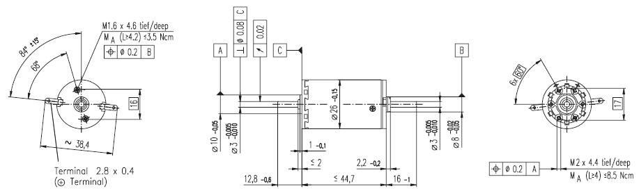
5.4.1. Interface Box
The interface box’s main task is to make connection between the control box, sensor and the PC. Another task is the switching of the power supply unit. It is common, that the personal computers are running 24 hours a day. But an experimental set up can not be turned on all day long because of security reasons. The idea of using the personal computer as a remote controllable switch, come up to expectations. It is common that a computer is able to turn on itself remotely ( by Wake On LAN). This function is provided by the Power Supply Unit (PSU), which provides a standby voltage (+5V, max 0.5 mA) even if it is turned off. A normal PSU can also provide voltage for an experimental DC servo motor and controller. The PCI-1720 D/A output cards’ 3. channel is used for turning on and off the PSU in the interface box, which supplies the servo amplifier with energy. Turning on is made by holding the voltage on +2V, and turning off is with voltage of 0V. The standby voltage is used to keep the PSU off and as the PS ON pin is low active, a small circuit is needed to make the voltage change. The circuit diagram and a picture of the real circuit is shown in Figure 5-3. and Figure 5-4.
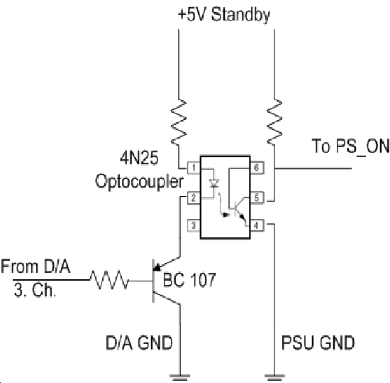
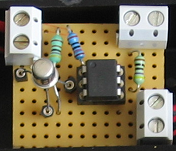
5.4.2. Parameters of the Planetary Gearhead
Planetary Geared straight teeth
Output shaft steel
Bearing at output ball bearings
Radial play, 5 mm
from flange max. 0.02 mm
Axial play 0.1 mm
Max. perm. radial load,
12.5 mm from flange 40 N
Max. permissible axial load 20 N
Max. permissible force
for press fits 20 N
Recommended input speed < 5000 rpm
Recommended
temperature range -30/+90°C
Number of stages 1 2 3
Average backlash no load<20‘<35‘<50‘
Gearhead data:
1 Reduction 33:1
2 Reduction absolute 299/9
3 Number of stages 2
4 Max. continuous torque
at gear output0.7 Nm
5 Intermittently permissible torque
at gear output 2.0 Nm
6 Sense of rotation, drive to output =
7 Max. efficiency 85 %
8 Weight 107 g
9 Gearhead length L1 36.7 mm
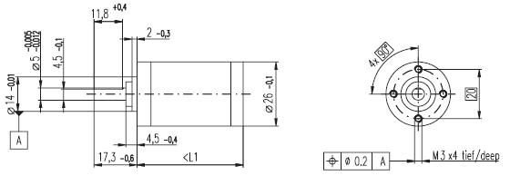
Technical data:
Supply voltage 5 V ± 10 %
Output signal EIA RS 422
Drivers used:DS26LS31
No. of channels 2+1 Index
Counts per turn500
Phase shift
Φ (nominal) 90°e
Logic state width s min. 45°e
Signal rise time180 ns
(typical at CL=25 pF, RL=2.7 kΩ, 25°C)
Signal fall time40 ns
(typical at CL=25 pF, RL = 2.7 kΩ, 25°C)
Index pulse width
(nominal) Option 90°e
Operating temperature range 0 / +70°C
Moment of inertia
of code wheel ≤ 0.6 gcm2
Max. acceleration 250 000 rad s-2
Output current per channel min. -1 mA,
max. 20 mA
Max. operating frequency 100 kHz
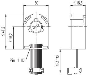
5.5. General guidelines to experiments
Every exercise can be reached through the homepage of the experiments address. The order of the exercises is defined in such a way that helps the users to build them on the results of the previous exercises. The layout of the homepage can be seen in Figure 5-7.

To reach an exercise, select it from the menu or the dropdown list as seen in Figure 5-8.

After reading the exercise instructions and the available additional help files, sources; the program controlling the system components can be written in the specified fields. The programming language is C++ and the variables and code can be inserted in two different input fields as seen in Figure 5-9.
|
|
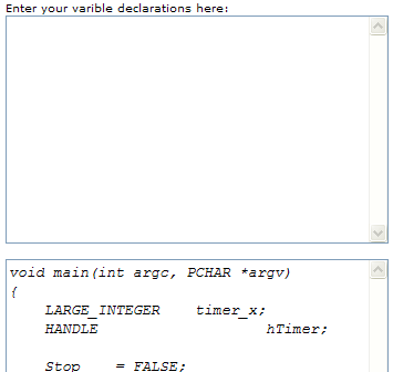
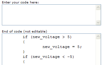
Figure 5-9. Solution input
To execute the experiment click the “Upload” button, placed at the bottom of the homepage.
If the solution is correct, the result of the exercise can be downloaded / observed.
Every exercise has different results. They can be observed and evaluated on the PC monitor by:
Webcam (e.g. video picture);
MATLAB files (e.g. position, voltage, velocity, time);
Graphs (e.g. position, voltage, velocity versus time).
Example of output is shown in
Experiment is complete!
Click to show time-time graph![]()
Click to show time-position graph![]()
Click to hide time-velocity graph![]()
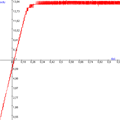
Click to show time-torque graph![]() Select item to download:
Select item to download:
5.6. Using the PCI-1720 D/A card – Motion control/ Exercise 1.
Every PC based measurement starts with opening a communication channel outside the PC itself. In case of the motor control the starting point is the control of a Digital-Analog converter card. This card enables us to send specified voltages from the PC to the measured system. The card has a programming interface (a DLL, Dynamic-Link Library), which can be called through C++ language. The DLL is already preloaded; only the function calls must be implemented.
The card is manufactured by Advantech Inc. and has a code PCI-1720. It has 4 output channels of D/A converters with an output range of -5V to +5V. Your task is to set the output voltage level of the D/A card channel 3 to 5 Volts. Actually, this 5 Volts enables the operation of the servo drive.
Steps needed:
Compare the “Advantech specific variables” in the framework program and in the sample program. Find the variables, which are changed.
Initialize the card (cut and paste step 3 and step 4 from the sample program).
Modify the variables, which are changed.
Remove the parts which are not relevant (printf(); and getch(); commands, which are used for printing a text and getting a character).
Set (output) the voltage (5 volts to channel 3).
5.6.1. Initializing the PCI-1720 card by the function: DRV_DeviceOpen
Function call: status = DRV_DeviceOpen(DeviceNum, DriverHandle)
Purpose: Retrieves parameters pertaining to operation of the device from the Registry or Configuration file, and allocate memory to store it for quick reference. This function must be called before any other functions.
Name | Direction | Type | Range | Description |
DeviceNum | Input | unsigned long | default | device number |
DriverHandle | Output | Long pointer | default | a pointer to the configuration data for the device |
Return:
SUCCESS if successful.
MemoryAllocateFailed if memory allocation failure.
ConfigDataLost if retrieving configuration data failure.
CreateFileFailed if low level driver has an opening failure.
Notes:
All subsequent functions perform the desired I/O operations based on configuration data retrieved by the DriverHandle parameter.
After the I/O operations, user has to call DRV_DeviceClose to release the memory allocated by DRV_DeviceOpen.
5.6.2. Setting the voltage level on PCI 1720 card by the function: DRV_AOVoltageOut
Function call: status = DRV_AOVoltageOut(DriverHandle, lpAOVoltageOut)
Purpose: Accepts a floating-point voltage value, scales it to the proper binary number, and writes that number to an analog output channel to change the output voltage.
Name | Direction | Type | Range | Description |
DriverHandle | Input | long | default | assigned by DRV_DeviceOpen |
lpAOVoltageOut | Input/Output | long pointer to PT_AOVoltageOut | default | the storage address for chan and OutputValue |
Return:
SUCCESS if successful.
InvalidDriverHandle if DriverHandle = NULL.
InvalidChan if input channel is out of range.
BoardIDNotSupported if this function is not supported for this Device.
5.6.3. Sample program of initializing and setting the voltage level on PCI-1720 card
NOTE
The names of the parameters used in this example are different from the names used in the actual measurement. You cannot simply cut and paste the parts of this example.
/*
***************************************************************************
 * Program        : DASOFT.CPP                       .                    *
 * Description    : Demo program for analog output function               *
 * Boards Supp.   : PCL-818 series/818HG/1800/816/812PG/711B/726/727/728, *
 *                  PCI-1710/1720, MIC-2728, ADAM-4021/5024               *
 * APIs used : DRV_DeviceOpen,DRV_DeviceClose, DRV_GetErrorMessage        *
 *                  DRV_AOVoltageOut                                      *
 * Revision       : 1.00                                                  *
 * Date           : 7/8/1999                   Advantech Co., Ltd.        *
 **************************************************************************
*/
#include <windows.h>
#include <windef.h>
#include <stdio.h>
#include <conio.h>
#include "..\..\..\include\driver.h"
/******************************
 * Local function declaration *
 ******************************/
void ErrorHandler(DWORD dwErrCde);
void ErrorStop(long*, DWORD);
void main()
{
    DWORD  dwErrCde;
    ULONG  lDevNum;
    long   lDriverHandle;
    USHORT usChan;
float  fOutValue;
PT_AOVoltageOut tAOVoltageOut;
    //Step 1: Display hardware and software settings for running this example
    printf("Before running this example, please\n");
    printf("use the device installation utility to add the device.\n");
    //Step 2: Input parameters
    printf("\nPlease input parameters:");
    printf("\nDevice Number (check the device installation utility): ");
    scanf("%d", &lDevNum);
    printf("\nOutput Channel: ");
    scanf("%d", &usChan);
    printf("\nOutput Value: ");
    scanf("%f", &fOutValue);

    //Step 3: Open device
    dwErrCde = DRV_DeviceOpen(lDevNum, &lDriverHandle);
    if (dwErrCde != SUCCESS)
    {
        ErrorHandler(dwErrCde);
        printf("Program terminated!\n");
        printf("Press any key to exit....");
        getch();
        exit(1);
    }
    // Step 4: Output value to the specified channel
    tAOVoltageOut.chan = usChan;
    tAOVoltageOut.OutputValue = fOutValue;
    dwErrCde = DRV_AOVoltageOut(lDriverHandle, &tAOVoltageOut);
    if (dwErrCde != SUCCESS)
    {
        ErrorStop(&lDriverHandle, dwErrCde);
        printf("Press any key to exit....");
        getch();
        return;
    }
    // Step 5: Display ouptut data
    printf("\nOutput data = %f\n", fOutValue);
    // Step 6: Close device
    dwErrCde = DRV_DeviceClose(&lDriverHandle);
    printf("\nPress any key to exit....");
    getch();
}//main
/**********************************************************************
 * Function: ErrorHandler
 *           Show the error message for the corresponding error code
 * input:    dwErrCde, IN, Error code
 * return:   none
 **********************************************************************/
void ErrorHandler(DWORD dwErrCde)
{
    char szErrMsg[180];
    DRV_GetErrorMessage(dwErrCde, szErrMsg);
    printf("\nError(%d): %s\n", dwErrCde & 0xffff, szErrMsg);
}//ErrorHandler
/**********************************************************************
 * Function:   ErrorStop
 *             Release all resource and terminate program if error occurs
 * Paramaters: pDrvHandle, IN/OUT, pointer to Driver handle
 *             dwErrCde, IN, Error code.
 * return:     none
 **********************************************************************/
void ErrorStop(long *pDrvHandle, DWORD dwErrCde)
{
    //Error message
    ErrorHandler(dwErrCde);
    printf("Program terminated!\n");

    //Close device
    DRV_DeviceClose(pDrvHandle);
}//ErrorStop
5.7. Using the real-time clock with PCI 1720 D/A card – Motion control/ Exercise 2.
The second important function in a PC based measurement is sampling. For this reason we need a real-time clock that can initiate the sampling at a specified moment and by a given frequency. There are several real-time operation systems including a real-time clock for synchronization. The multitask type Windows Operation System does not support the real time applications but the Real-Time eXtension (RTX) for Control of Windows solves that problem. You can read a description on it below but you do not need to understand its operation fully for this measurement. The application of the real-time clock is tested in Exercise 2.
A clock is ticking in the program given in the exercise (every millisecond) and your task is to output a sinusoidal voltage time function (3 Volts amplitude and 1 Hz frequency) by the PCI 1720 D/A card. .
You have to define the relationship of the sampling time and the sine wave. The sampling time starts from 0 and can be reached through the CurrentTime variable given in the program. This time variable can be reached through the variable time_array[tickCount] and the value is given in 100 nanosecond units.
Steps needed:
Study the given program framework
Write in the missing codes
Declare the parameters and variables
Out=Amplitude * sin (Angular Frequency *time) (Note it is not a C code and you have to read time by the TimerHandler function)
5.7.1. How real-time is achieved without real-time operating system?
(Just to read)
Real-Time eXtension (RTX) for Control of Windows is specifically designed as an optimized extension to the Windows operating system. It is not a Real-Time Operating System (RTOS) ported to Windows. RTX provides precise control of IRQs (Interrupt ReQuests), I/O, and memory to ensure that specified tasks are executed with proper priority and 100% reliability. By operating in Ring 0, RTX ensures the highest performance and requires minimal configuration, supporting sustained interrupt rates of 30 KHz with an average IST latency of less than one microsecond. RTX is a true Windows extension, utilizing all the standard Windows conventions, including the APIs, memory management, SRIs, mutexes, and semaphores familiar to Windows developers. An RTX application can take full advantage of the memory-protection mechanisms offered by Windows and the Intel architecture in Ring 3. Once the developer completes debugging and ensures that memory pointers and arrays are valid, the RTX application can immediately be recompiled to run in Ring 0 for optimum performance. The key is in architecture, which can be seen in Fig. 6.
RTX architecture is a true extension in that it does not encapsulate Windows and does not interfere with, or modify any of the Windows infrastructure. By maintaining this separation, the RTX real-time sub-system (RTSS) ensures that RTX-based applications survive Windows crashes or “blue screens.” The RTX RTSS kernel is designed around a high-speed scheduler that utilizes both preemptive and round-robin algorithms. RTX supports up to 1,000 independent processes, with each process supporting unlimited threads. Fine-grained control over applications is assured with 256 levels of assignable thread priority. The scheduler guarantees that critical thread context switches and yields to threads of higher priority occur in the 500 nanosecond to less than two microsecond range. To facilitate data communications between RTX processes and Win32 applications, RTX utilizes a high-throughput messaging and synchronization IPC mechanism. Using a shared memory model, IPC can transfer large amounts of data with no performance degradation. Precise execution of events is critical in a real-time system. To support this precision, RTX provides three clocks on which to base event timers. Clock resolution, depending on the clock used, can be precise within 0.001 nanosecond, without any drift.
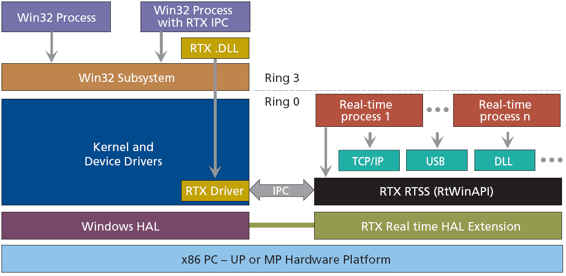
5.8. Using the PCI-1784 Counter card – Motion control/ Exercise 3.
The counter is used to read the signal of the encoder and convert it to a numeric representation. The counter value is read by TimerHandler function, which is executed in every tick of the real-time clock.
Your task is to read the counter value of channel 3 on the PCI-1784 card.
Steps needed:
Initialize the card.
Reset counter values.
Start counting operation.
Read counter value in the beginning.
Read counter value at every tick of real-time clock.
5.8.1. Initializing the PCI-1784 card by the function of DRV_DeviceOpen (see Exercise 1.)
Function call: status = DRV_DeviceOpen(DeviceNum, DriverHandle)
Purpose: Retrieves parameters pertaining to the operation of the device from the Registry or configuration file, and allocate memory to store it for quick reference. This function must be called before any other functions.
Name | Direction | Type | Range | Description |
DeviceNum | Input | unsigned long | Default | device number |
DriverHandle | Output | long pointer | default | a pointer to the configuration data for the device |
Return:
SUCCESS if successful.
MemoryAllocateFailed if memory allocation failure.
ConfigDataLost if retrieving configuration data failure.
CreateFileFailed if low level driver has an opening failure.
Notes:
All subsequent functions perform the desired I/O operations based on configuration data retrieved by the DriverHandle parameter.
After the I/O operations, user has to call DRV_DeviceClose to release the memory allocated by DRV_DeviceOpen.
5.8.2. Reset counter values on PCI-1784 card by the function: DRV_CounterReset
Function call: status = DRV_CounterReset(DriverHandle, counter)
Purpose: Turns off the specified counter operation.
Name | Direction | Type | Range | Description |
DriverHandle | Input | long | Default | assigned by DRV_DeviceOpen |
counter | Input | long | Default | counter channel |
Return:
SUCCESS if successful.
InvalidDriverHandle if DriverHandle = NULL.
BoardIDNotSupported if the function is not supported for this device.
InvalidChannel if the port number is out of range.
5.8.3. Start counting operation on PCI-1784 card by the function of DRV_CounterEventStart
Function call: status = DRV_CounterEventStart(DriverHandle, lpCounterEventStart)
Purpose: Configures the specified counter for an event-counting operation and starts the counter.
Name | Direction | Type | Range | Description |
DriverHandle | Input | long | default | assigned by DRV_DeviceOpen |
LpCounterEventStart | Input/Output | long pointer to PT_CounterEventStart | default | the storage address for countger and GateMode |
Return:
SUCCESS if successful.
InvalidDriverHandle if DriverHandle = NULL.
BoardIDNotSupported if the function is not supported for this device.
InvalidChannel if the port number is out of range.
Operations:
The programming method depends on the counter/timer chip on the board. There are two kinds of chips used in A/D Card: Intel 8254 and AMD Am9513A. For Am9513A, counter channels 0-9 can all function as a rising edge event counter. Connect your external event generator to the clock input of the desired counter. If hardware ”gating”, in which the counter may be started by a separate external hardware input, is desired, choose a gating type and use an external device to trigger the gate input of the counter.
Both of the above counter/timer chips are 16-bits. However, the function supports a 32-bit counter, i.e. it counts up 232. It will check if the counter is overflowing and converts it to 32-bits by calculation.
Intel 8254 hardware counter needs 2 cycle time to reload counter setting, so counter program has to wait for 2 external trigger (cycle time) to read correct counter value. At the first time of calling ”DRV_CounterEventStart”, Intel 8254 hardware uses default value to initialize its counter setting. This initialization will take about 2 external trigger (cycle time) to finish. If ”DRV_CounterEventRead” is called before initialization is finished, then the program will get incorrect value. So, you have to delay 2 external trigger (cycle time) in program before calling ”DRV_CounterEventRead” to make sure the return value is correct. The delay time is dependent of the time of external trigger.
5.8.4. Read counter values on PCI-1784 card by the function of DRV_CounterEventRead
Function call: status = DRV_CounterEventRead(DriverHandle, lpCounterEventRead)
Purpose: Reads the current counter total without disturbing the counting process and returns the count and overflow conditions.
Name | Direction | Type | Range | Description |
DriverHandle | Input | long | default | assigned by DRV_DeviceOpen |
lpCounterEventRead | Input/Output | long pointer to PT_CounterEventRead | default | the storage address for counter, overflow and count |
Return:
SUCCESS if successful.
InvalidDriverHandle if DriverHandle = NULL.
BoardIDNotSupported if the function is not supported for this device.
InvalidChannel if the port number is out of range.
5.8.5. Sample program of counter operations on PCI-1784 card
NOTE
The names of the parameters used in this example are different from the names used in the actual measurement. You cannot simply cut and paste the parts of this example.
/*
***************************************************************************
 * Program        : COUNTER.CPP                                           *
 * Description    : Demo program for counter function                     *
 * Boards Supp.   :                                                       *
 * APIs used      : DRV_DeviceOpen,DRV_DeviceClose, DRV_GetErrorMessage,  *
 * DRV_CounterReset, DRV_CounterEventStart, DRV_CounterEventRead          *
 * Revision       : 1.00                                                  *
 * Date           : 7/8/1999                   Advantech Co., Ltd.        *
***************************************************************************
#include <windows.h>
#include <windef.h>
#include <stdio.h>
#include <conio.h>
#include "..\..\..\..\include\driver.h"
/******************************
 * Local function declaration *
 ******************************/
void ErrorHandler(DWORD dwErrCde);
void ErrorStop(long*, DWORD);
void main()
{
    DWORD  dwErrCde;
    ULONG  lDevNum;
    long   lDriverHandle;
    USHORT wChannel = 0;
USHORT wOverflow = 0;         // counter over 32 bit flag
ULONG  dwReading = 0;
PT_CounterEventStart tCounterEventStart;
    PT_CounterEventRead  tCounterEventRead;
    //Step 1: Display hardware and software settings for running this example
    printf("Before running this example, please\n");
    printf("use the device installation utility to add the device.\n");
    //Step 2: Input parameters
    printf("\nPlease input parameters:");
    printf("\nDevice Number (check the device installation utility): ");
    scanf("%d", &lDevNum);
    printf("\nInput Channel: ");
    scanf("\n%d", &wChannel);
    //Step 3: Open device
    dwErrCde = DRV_DeviceOpen(lDevNum, &lDriverHandle);
    if (dwErrCde != SUCCESS)
    {
        ErrorHandler(dwErrCde);
        printf("Program terminated!\n");
        printf("Press any key to exit....");
        getch();
        exit(1);
    }
    // Step 4: Reset counter by DRV_CounterReset
dwErrCde = DRV_CounterReset(lDriverHandle, wChannel);
    if (dwErrCde != SUCCESS)
    {
        ErrorHandler(dwErrCde);
        printf("Program terminated!\n");
        printf("Press any key to exit....");
        getch();
        exit(1);
    }
    // Step 5: Start counting operation by DRV_CounterEventStart
tCounterEventStart.counter = wChannel;
    dwErrCde = DRV_CounterEventStart(lDriverHandle, &tCounterEventStart);
    if (dwErrCde != SUCCESS)
    {
        ErrorHandler(dwErrCde);
        printf("Program terminated!\n");
        printf("Press any key to exit....");
        getch();
        exit(1);
    }
    // Step 6: Read counter values by DRV_CounterEventRead in while loop
    //         and display counter value, exit when pressing any key
tCounterEventRead.counter = wChannel;
    tCounterEventRead.overflow = &wOverflow;
    tCounterEventRead.count = &dwReading;
    while( !kbhit() )
    {
       dwErrCde = DRV_CounterEventRead(lDriverHandle, &tCounterEventRead);
       if (dwErrCde != SUCCESS)
       {
          ErrorStop(&lDriverHandle, dwErrCde);
          return;
       }
       printf("\nCounter value = %lu", dwReading);
       Sleep(1000);
    }
    // Step 7: Stop counter by DRV_CounterReset
dwErrCde = DRV_CounterReset(lDriverHandle, wChannel);
    if (dwErrCde != SUCCESS)
    {
        ErrorHandler(dwErrCde);
        printf("Program terminated!\n");
        printf("Press any key to exit....");
        getch();
        exit(1);
    }
    // Step 8: Close device
    dwErrCde = DRV_DeviceClose(&lDriverHandle);
    getch();
    printf("\nPress any key to exit....");
    getch();
}//main
/**********************************************************************
 * Function: ErrorHandler
 *           Show the error message for the corresponding error code
 * input:    dwErrCde, IN, Error code
 * return:   none
 **********************************************************************/
void ErrorHandler(DWORD dwErrCde)
{
    char szErrMsg[180];
    DRV_GetErrorMessage(dwErrCde, szErrMsg);
    printf("\nError(%d): %s\n", dwErrCde & 0xffff, szErrMsg);
}//ErrorHandler
/**********************************************************************
 * Function:   ErrorStop
 *             Release all resource and terminate program if error occurs
 * Paramaters: pDrvHandle, IN/OUT, pointer to Driver handle
 *             dwErrCde, IN, Error code.
 * return:     none
 **********************************************************************/
void ErrorStop(long *pDrvHandle, DWORD dwErrCde)
{
    //Error message
    ErrorHandler(dwErrCde);
    printf("Program terminated!\n");

    //Close device
    DRV_DeviceClose(pDrvHandle);
    printf("Press any key to exit....");
    getch();
    exit(1);
}//ErrorStop
5.9. Open Loop Control measurement – Motion control/ Exercise 4.
After the introduction of the PC based measurement system, it is time for writing the first controller for a DC motor.
5.9.1. Theoretical background for DC servomotor
The theoretical background is overviewed in substantial number of animated slides. Additional explanation can be accessed from the animated slides. This is a compressed repetition of the DC motor module of a PC based material entitled “INETELE Interactive and Unified E-Based Education and Training for Electrical Engineering”.
5.9.2. Construction and equivalent circuit of DC servomotor
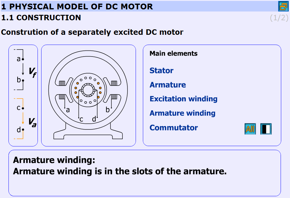
The construction of the DC-servo motor:
Stator: Stator is the stationary part of the machine.
Armature: Armature is the rotating part of the machine.
Excitation winding: Excitation winding is placed around the poles in the stator.
Armature winding: Armature winding is in the slots of the armature.
Commutator: The commutator periodically reverses the current. It consists of rotating segmented copper contacts and stationary carbon brushes.
Equivalent circuit
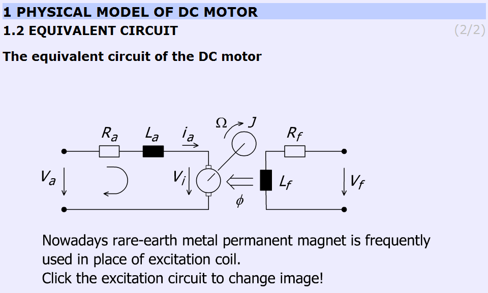
Parameters and variables of the DC servomotor:
Ra – Armature resistance [ohm];
La – Armature inductance [henry];
J – Inertia [kgm2];
va – Armature voltage [volt];
vi – Back e.m.f. generated in the armature winding [volt];
ia – Armature current [ampere];
Ω – Shaft speed of the motor [rad/s];
Vf, Rf, Lf, Ф are pertaining to the excitation circuit.
This subchapter focuses on the excitation of the DC motor. In most cases in the small DC motors permanent magnet is applied.
5.9.3. Mathematical model
This chapter explains the mathematical model of the DC motor. Three main parts can be found here:
Time-domain equations
Frequency-domain equations
Transfer functions
Time-domain equations
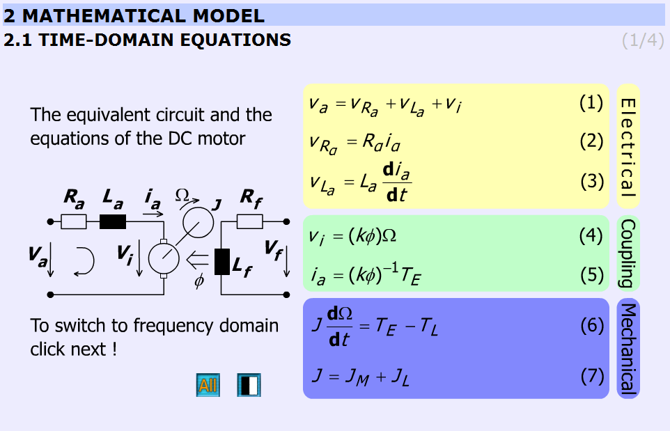
This chapter presents the time-domain equations. These slides are focused on the following equations:


where  is the electric torque of the motor
| (5.6) |

where  is the torque of the load
| (5.7) |

where  is the load inertia.
The explanation can be found in the “INETELE Interactive and Unified E-Based Education and Training for Electrical Engineering”. It can be reached from the slide shown in Figure 5-15. It contains the bridge to the next frame declining with the frequency-domain equations.
Frequency-domain equations
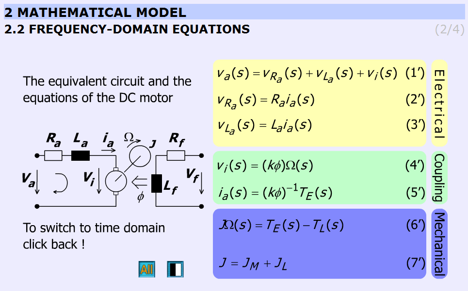
This chapter presents the frequency-domain equations. The variables are complex quantities (s = jω).
| (5.10) |
| (5.11) |
| (5.12) |
| (5.13) |
| (5.14) |

Transfer functions
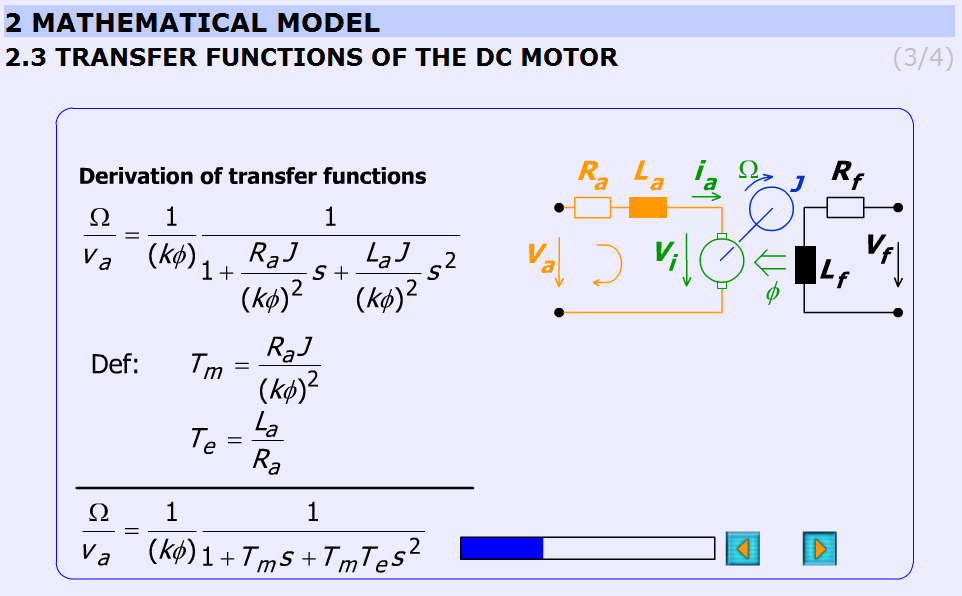
This subchapter explains the derivation of the transfer function of the DC motor in a detailed form step-by-step.
The initial equations are given in the previous chapter (Frequency-domain equations) and the final equations are:
The electrical, Te and mechanical, Tm time constants are:


The animation contains explanation images as well. Images are changing according to the derivation stages. The progress bar graphically shows the percentage of the derivation completed.
The derivation of the time constants can be seen in Figure 5-17.
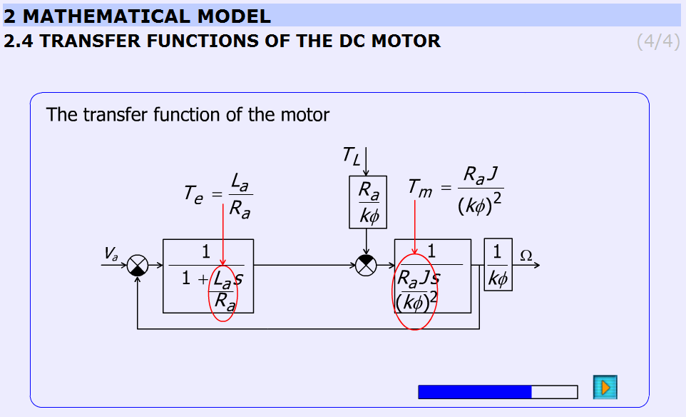
5.9.4. Analysis of the model
State space representation
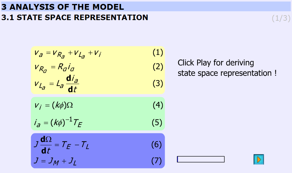
This subchapter derives the state space representation in the same way as in the subchapter Transfer functions of the DC motor was done. The initial conditions are the same as in the subchapter Time-domain equations. The result is the following:
| (5.19) |
Using vectors and matrices the state space representation:
| (5.20) |

where x is the state vector.
Steady state
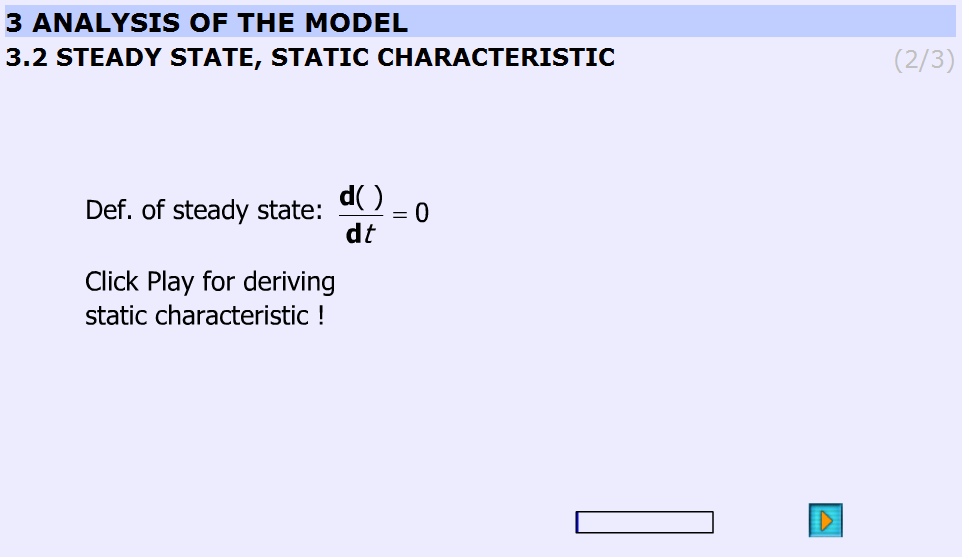
This subchapter derives the static characteristic equation of the DC motor in steady state operation. On that basis the next subchapter the static characteristics will show.
The derivation starts with the assumption:
| (5.21) |

and ends with
( | (5.22) |

| (5.23) |
Static characteristic, working point
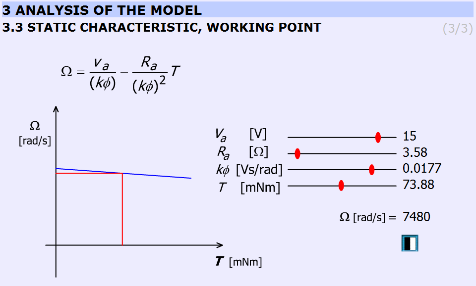
This subchapter explains the static characteristics and the working point.
The basic equation of the animation:
| (5.24) |

(26)
The Simulink model of the Maxon motor used in the experiment is based on its rated values. They are the followings:
( | (5.25) |

( | (5.26) |

( | (5.27) |

( | (5.28) |


The gear ratio: 33/1
The blue line is the static characteristic of the motor. The cross-section of the red line with the motor characteristics yields the working point. The rated values are indicated by vertical lines on the sliding bar.
5.9.4.1. Analysis of the transfer function
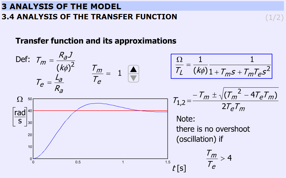
The transient response of the DC motor is discussed for step wise load torque change using different  ratio. The possibility of overshoot is explained. By changing
  , the response will also change. The time functions are calculated and uploaded. The ratio
  can be varied only in discrete predefined steps.
The equation to be solved:
( | (5.38) |
The ratio can be varied in steps: 1; 2; 4; 8; 16; 33; 66.
The explanation is based on the roots of the characteristic equation:
( | (5.39) |
Two real roots exist if  . The border case is:
( | (5.40) |
than
When  conjugate complex roots are obtained.
The simulation was carried out by using MatLab Simulink. The simulation setup can be seen in Figure 5-22.
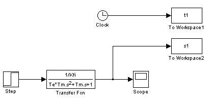
Analysis of the transfer function
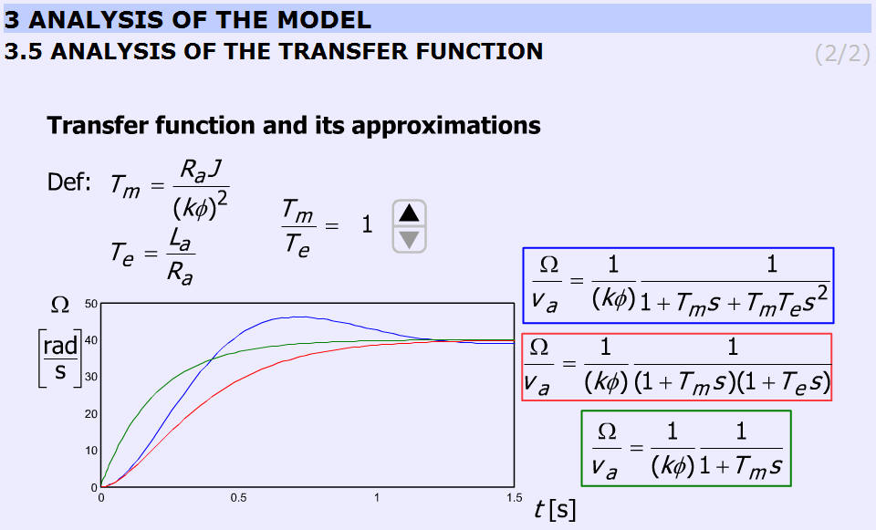
This subchapter explains the deviations among approximations taking into consideration the ratio  . The animation is built up exactly in the same way as in the previous chapter. The ratio
  can be varied in steps: 1; 2; 4; 8; 16; 33; 66.
Comparison with the previous chapter is also possible.
The accurate equation and its approximations:
The simulation was carried out by using MatLab Simulink. The simulation setup can be seen in Figure 5-24.
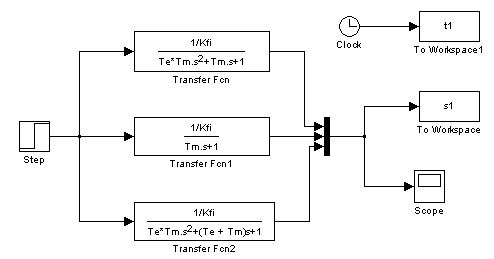
5.9.5. Digital filter
After the introduction of the PC based measurement system, it is time for writing the first controller for a DC motor.
The time function of velocity is very noisy. A smooth curve can be obtained from the noisy signal by low pass filtering in the following way. Let the input of the system be the measured velocity,  , and the output of the system is the filtered velocity,
| (5.46) |

Appling three serial connected lowpass filters with time constant  . The transfer function of the filter is
| (5.47) |
After rearrangement
| (5.48) |

Inverse Laplace-transformation
| (5.49) |

where Tc is the time period of the cut off frequency and the dot (  ) is short for derivate with respect to time. The state space equation of the filter is
| (5.50) |
The state space equation (5.50) can be rewrite in a Discrete time form.
| (5.51) |
Where k is short for the kth sampling and the elements of the system matrix (ai and bi) can be calculated by the MATLAB function “c2d”, which is short for “continuous to discrete”.
[Ad, Bd] = c2d(A, B, tsample);
where tsample is the sampling period and Tc is the time constant of the filter.
Draft calculation of the filter cut off angular frequency
| (5.54) |
The filter parameter
| (5.55) |
A MATLAB script is created to calculate and print the filter parameters. It was necessary to check differences between filters. A third order Bessel filter and a fifth order Bessel filter are created.
.
The MATLAB script for calculation of discrete time filter parameters:
Ts = 0.001;
Tc = 10*Ts;
A = [0, 1, 0;
0, 0, 1;
-1/Tc^3, -3/Tc^2, -3/Tc];
B = [0;0;1/Tc^3];
[Ad,Bd] = c2d(A,B,Ts);
for i = 1:3
for j = 1:3
disp(['float ad',num2str(i),num2str(j),' = ', num2str(Ad(i,j)),';']);
end
end
for i = 1:3
disp(['float bd',num2str(i),' = ', num2str(Bd(i)),';']);
end
Result
float ad11 = 0.99591;
float ad12 = 0.00095987;
float ad13 = 3.652e-007;
float ad21 = -11.3235;
float ad22 = 0.88778;
float ad23 = 0.00061567;
float ad31 = -19089.6748;
float ad32 = -193.6165;
float ad33 = 0.30752;
float bd1 = 0.0040906;
float bd2 = 11.3235;
float bd3 = 19089.6748;
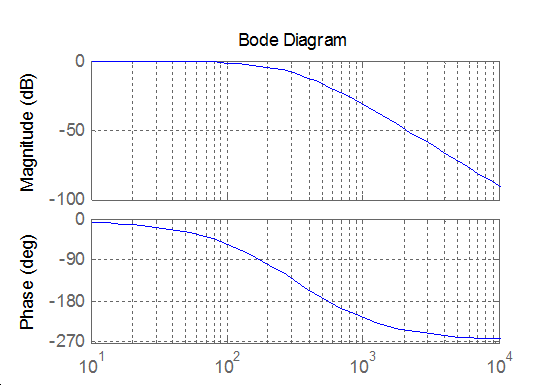
The transfer function of a third order Bessel filter:
| (5.56) |
The MATLAB script for calculation of discrete time filter parameters:
Ts = 0.001;
Tc = 1/(2*pi*1/(2*Ts)/10);
A = [0, 1, 0;
     0, 0, 1;
     -15/Tc^3, -15/Tc^2, -6/Tc];

B = [0;0;15/Tc^3];

[Ad,Bd] = c2d(A,B,Ts);

for i = 1:3
    for j = 1:3
        disp(['float ad',num2str(i),num2str(j),' = ',num2str(Ad(i,j)),';'])
    end
end

for i = 1:3
    disp(['float bd',num2str(i),'  = ', num2str(Bd(i)),';']);
end
Result
float ad11 = 0.95193;
float ad12 = 0.00083371;
float ad13 = 2.6009e-007;
float ad21 = -120.9668;
float ad22 = 0.56688;
float ad23 = 0.00034345;
float ad31 = -159737.83;
float ad32 = -629.4281;
float ad33 = -0.080513;
float bd1  = 0.048071;
float bd2  = 120.9668;
float bd3  = 159737.83;
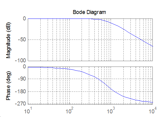
The transfer function of a fifth order Bessel filter
| (5.57) |
The MATLAB script for calculation of discrete time filter parameters:
Ts = 0.001;
Tc = 1/(2*pi*1/(2*Ts)/10);
A = [0, 1, 0, 0, 0;
     0, 0, 1, 0, 0;
     0, 0, 0, 1, 0;
     0, 0, 0, 0, 1;
     -945/Tc^5, -945/Tc^4, -420/Tc^3, -105/Tc^2, -15/Tc];

B = [0;0;0;0;945/Tc^5];

[Ad,Bd] = c2d(A,B,Ts);

for i = 1:5
    for j = 1:5
        disp(['float ad',num2str(i),num2str(j),' = ',num2str(Ad(i,j)),';'])
    end
end

for i = 1:5
    disp(['float bd',num2str(i),'  = ', num2str(Bd(i)),';']);
end
Result
float ad11 = 2.3749;
float ad12 = 0.0060369;
float ad13 = 8.9952e-006;
float ad14 = 8.7509e-009;
float ad15 = -2.4834e-013;
float ad21 = -55.9541;
float ad22 = 0.80926;
float ad23 = 0.00070548;
float ad24 = 2.3492e-007;
float ad25 = 6.3994e-011;
float ad31 = -185062.4462;
float ad32 = -645.0082;
float ad33 = -0.024158;
float ad34 = 4.2341e-005;
float ad35 = 1.3387e-007;
float ad41 = -387151871.8085;
float ad42 = -1417349.3637;
float ad43 = -2388.3942;
float ad44 = -1.4113;
float ad45 = 7.4665e-005;
float ad51 = -215947384065.4345;
float ad52 = -1074421228.8149;
float ad53 = -2389749.1508;
float ad54 = -3161.8599;
float ad55 = -0.37582;
float bd1  = -1.3925e-005;
float bd2  = 0.00056689;
float bd3  = 1.8749;
float bd4  = 3922.0853;
float bd5  = 2186784.2468;
5.9.6. Description of the measurement
The CalculateController function is called every tick of the real-time clock.
#include <windows.h>
#include <stdio.h>
#include <rtapi.h>
#include <math.h>
#include <string.h>
#define PI 3.14159265358979323846
typedef struct
{
float Position;
float Velocity;
float Torque;
float StateVariable_5;
float StateVariable_6;
float StateVariable_7;
float StateVariable_8;
float StateVariable_9;
float StateVariable_10;
} NewControllerData;
NewControllerData CalculateController(
const float CurrentPosition,
const float OldPosition,
const float OldVelocity,
const float CurrentTime,
const float OldTime,
const float Old_StateVariable_5,
const float Old_StateVariable_6,
const float Old_StateVariable_7,
const float Old_StateVariable_8,
const float Old_StateVariable_9,
const float Old_StateVariable_10
)
{
NewControllerData ResultData; // result
//Declaration of your controller
// Position is saved automatically
ResultData.Position = CurrentPosition;
// Angular velocity is saved automatically
if (CurrentTime != 0.0f){
ResultData.Velocity = (1000.0f * (float)(CurrentPosition - OldPosition)/(float)(CurrentTime - OldTime));
}
else {
ResultData.Velocity = 0.0f;
}
//Calculation of your controller
return ResultData;
}
The new values of the variables and all calculations must be done inside this function. The state of the motor can be reached through the variables of the function:
ResultData.Position for the position;
ResultData.Velocity for the angular velocity of the motor;
ResultData.Time for the actual time.
For safety reasons, the input voltage of the motor cannot be set directly. The output of your controller program, which is the output signal of the D/A card is the reference current signal. You can consider it as a reference torque signal as well. This signal is defined as a variable named as
ResultData.Torque = …
The user should set the value at the end of “your controller program”. For example
ResultData.Torque = 1;
means that the torque of the shaft (after the gear) is set to 1 Nm. Since the output of the D/A card is voltage, the framework program calculates the proper voltage value from ResultData.Torque, which will be the output signal.
In this exercise Open Loop measurements will be performed with the DC motor. The user can select max 10 state variables to save in matlab form. Four of the 10 are fixed: time, position, angular velocity and the torque of the motor. If you want to save the state variable error you can do the following procedure.
Enter the name of the state variable vel_filt (filtered velocity) in to the fifth line like:
5. vel_filt;
Enter your variable declaration:
float vel_filt;
Enter the following in to your controller box
Vel_filt = (you have to calculate the value of the filtered velocity)
ResultData.StateVariable_5 = vel_filt;
After the measurement you can download the state variable vel_filt as well.
NOTE
The controller function is called in each sampling period. After finishing this function, all variables (except ResultData.Time, ResultData.Velocity, ResultData.Position ResultData.Torque and ResultData.StateVariable_5-10) are released (i.e. the values are lost). If you need a variable in the next sampling period you have to declare as static type variable. For example
static float vel_filt;
General steps needed:
Study the literature of DC motor overviewed in the current chapter entitled “Theoretical background for DC servo motor” below.
You can set the length of the measurement in millisecond (default value is 1000)
Based on measurements determine the transient responses and the steady-state characteristics of the DC servomotor.
As a help, the initialization of the two cards examined in Exercise 1-3 has already been performed for you. Only the above mentioned steps are needed for successful experiment.
5.9.7. Exercise tasks
Task 1.
In this exercise Open Loop measurements will be performed with the DC motor. Please, study the literature of DC motor overviewed in the current chapter below entitled “Theoretical background for DC servo motor”. In the first task, the electrical torque is set to
ResultData.Torque = 0.1;
ResultData.Torque = 0.5;
ResultData.Torque =1.0;
This way the step responses of various motor variables to different step change size in torque signals can be obtained. The result files, which can be downloaded at the end of the measurement, can be evaluated in Matlab. There is a program already written for this task. Running this program results in the shaft speed-time, voltage-time and position-time diagrams. These diagrams can also be saved in jpg format for further documentation.
Task 2. Digital filter
Task 3. Response of the motor to sinusoidal torque and compensation of the servo amplifier offset
The servo amplifier of has an offset voltage. This is the most obvious if we apply a sinusoidal voltage. In this case we expect the motor to have sinusoidal shaft speed and sinusoidal position change coming from the shaft speed.
5.10. Closed Loop Control Measurements – Motion control/ Exercise 5.
5.10.1. Theoretical background of Control theories
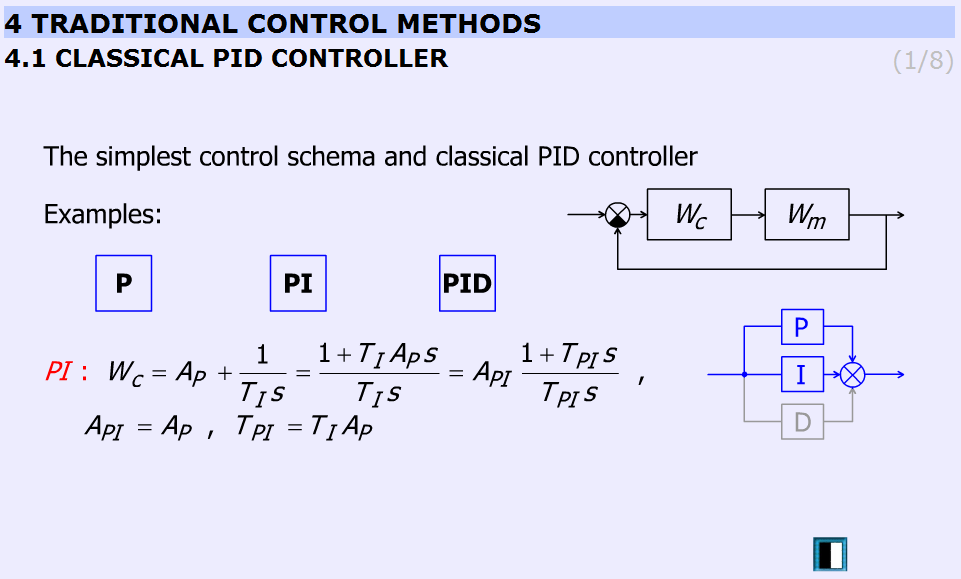
This animation presents the P, PI, PID controllers and the difference between them.
“P”:
( | (5.58) |

“PI”:
“PID”:
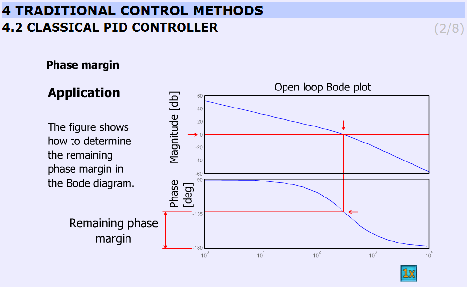
Figure 5-28. shows the application of the controller.
Animated explanation of the determination of the phase margin: On the Amplitude diagram on level 0, a red horizontal line appears. At the point, where the red line crosses the amplitude curve a vertical line goes down into the Phase diagram. The point, where this line crosses the phase curve, a horizontal line shows the actual phase. At the end the phase margin appears which can be calculated this way:
180o – actual phase = phase margin
This is indicated by the dimensional line on the phase axis.
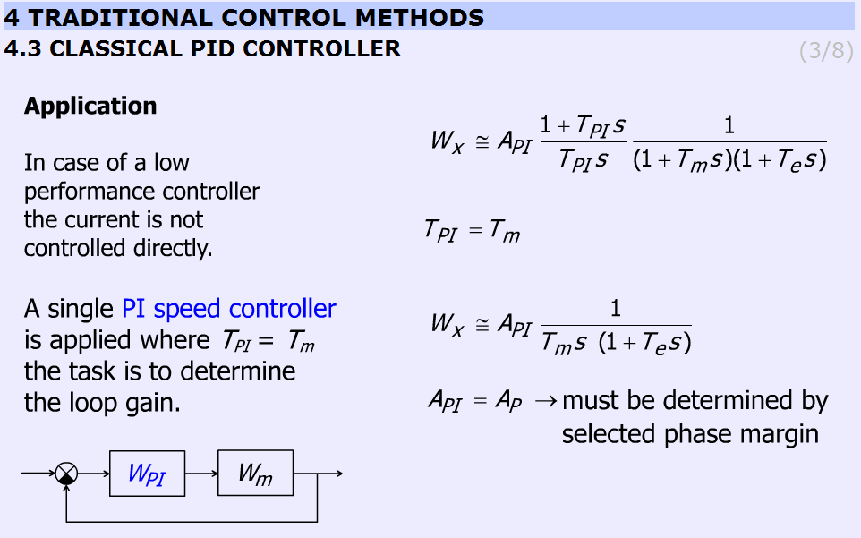
This slide explains the design applying PI controller. The transfer function of the controller and the motor with one approximation:
| (5.63) |
By selecting  the transfer function becomes:
| (5.64) |
Finally  and the task is to determine AP by choosing the phase margin.
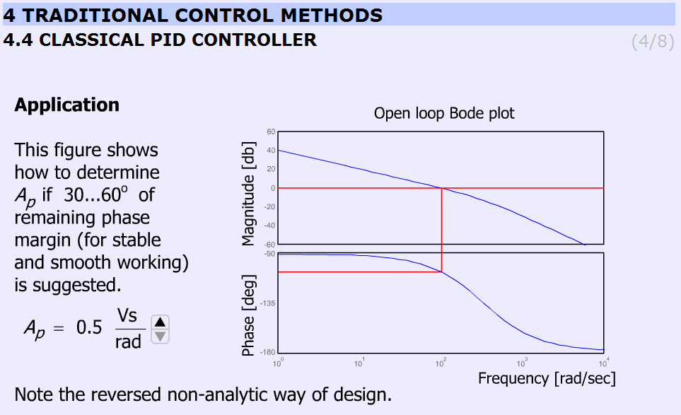
The animation shows the determination of Ap for 30...60o phase margin (for stable and smooth working) in a reversed non-analytical way, where the Bode plots let us to see the phase margin. The users can vary Ap between 0.5 and 3.5 and can check the effect of different gains on the phase margins. The animation uses the preliminary simulated results and graphs. Ap can be varied from 0.5 to 3.5 in 7 steps (0.5; 1.0; 1.5; 2.0; 2.5; 3.0; 3.5).
Parameters used in the simulation:
Tpi = 0.2 s;
Api = variable;
Kfi = 0.025 Vs/rad;
Te = 0.003 s;
Tm=Tpi.
MatLab commands:
g = tf([Api/Kfi],[Tpi*Te Tpi 0]);
bode(g);
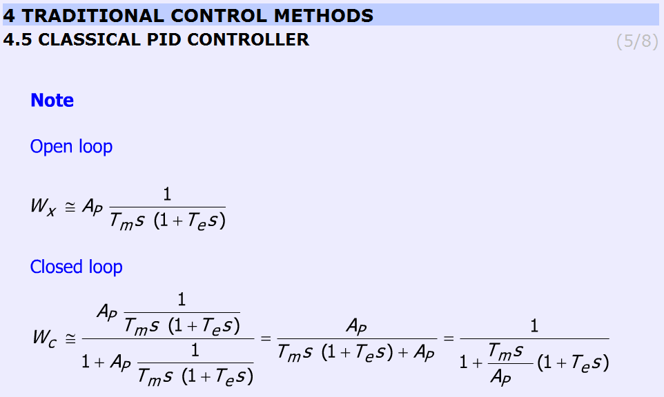
This slide helps to remember the open and the closed loop transfer function. The controller is PI ant TPI = Tm. The equations are as follows (without derivation):
Open loop
| (5.65) |
Closed loop
| (5.66) |
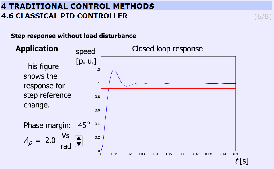
This animation presents the response for stepwise change in speed reference signal.
It should be noted that increasing Ap does not necessary result in overshoot. The animation uses the preliminary simulated results and graphs. Ap can be varied from 0.5 to 3.5 in 7 steps (0.5; 1.0; 1.5; 2.0; 2.5; 3.0; 3.5).
The simulation was carried out using MatLab Simulink. The simulation setup can be seen in Figure 5-33.
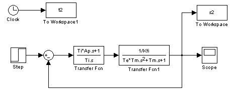
The arremgement of the motor and the PI controller in a feed-back loop can be seen in Figure 5-34.
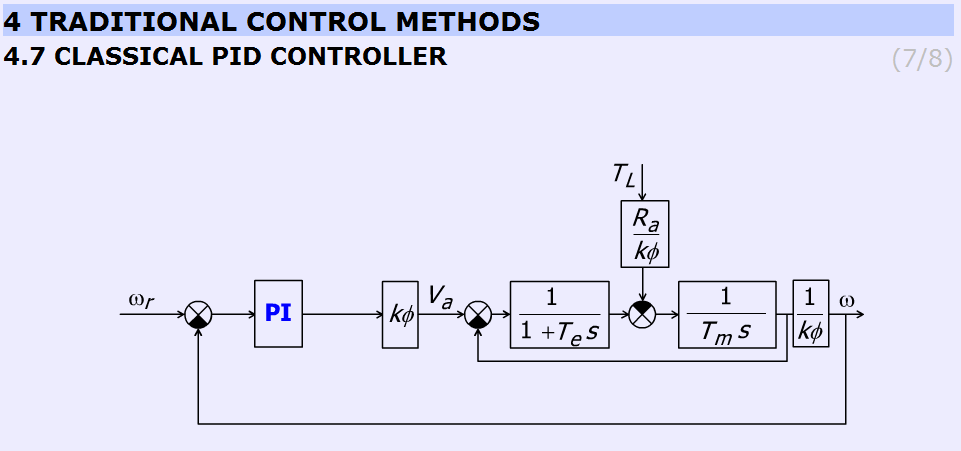
The user can observe that by increasing AP the overshot is getting higher.
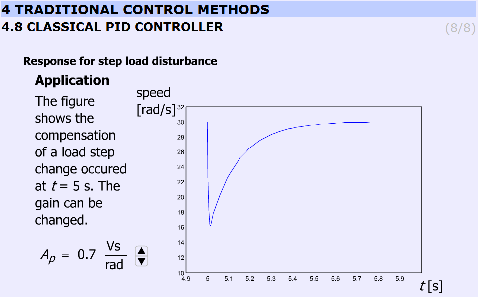
This slide (Figure 28) displays the effect of disturbance rejection. A stepwise load torque disturbance at t = 5s is at the input. The animation compares the speed of the controller at different Ap. Ap can be varied from 0.5 to 3.5 in 8 steps (0.5; 0.7; 1.0; 1.5; 2.0; 2.5; 3.0; 3.5). AP = 0.7 is included too because the difference between 0.5 and 1.0 is to significant.
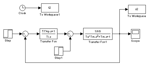
5.10.2. Current controller
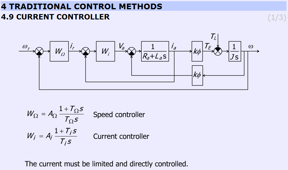
The subchapter entitled “current controller” explains the operation of the current controller briefly. The page contains a detailed block diagram of the motor and the controllers (speed and current) and the equations of the controllers
Speed controller:
| (5.67) |
Current controller:
| (5.68) |

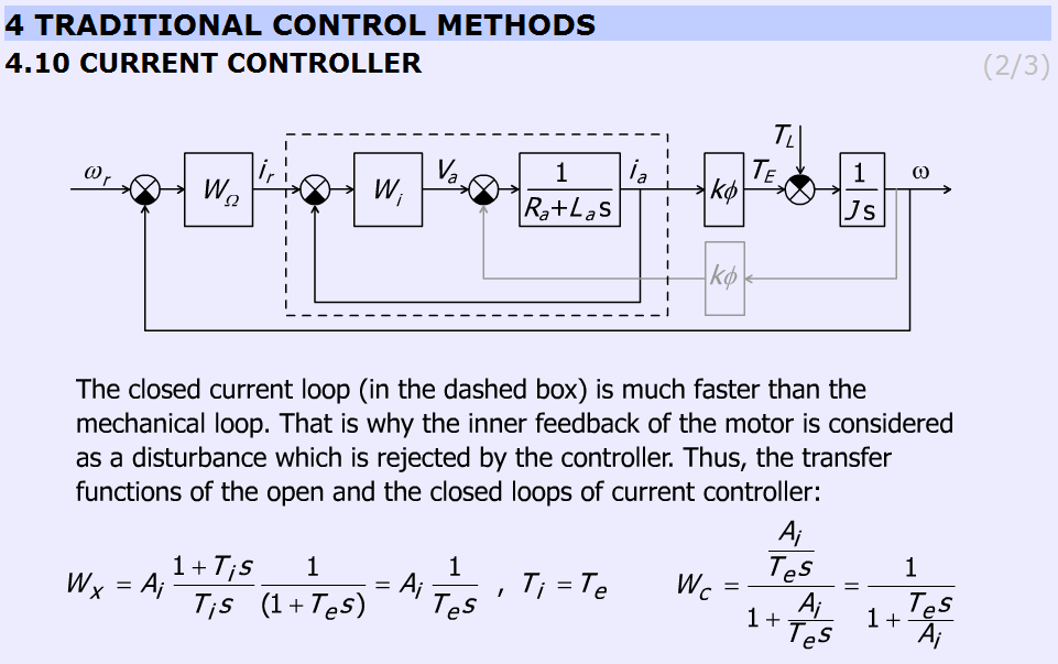
This slide explains why the internal feedback of the motor can be neglected. The figure helps to identify the more and less important elements. The internal feedback of the motor can be neglected because the current controller is much faster than the mechanical controller. Therefore, the internal feedback can be considered as a disturbance, which changes slowly, and this way the controller can eliminate the error caused by the inaccurate model of the DC motor.
The slide gives the equations to explain the operation of the controller.
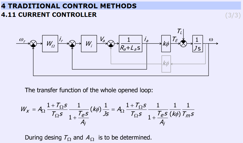
Figure 5-40 gives the open loop transfer function of the whole system.
| (5.69) |
where ωe = ωr – ω.
5.10.3. Methods for selecting the parameter values for PID controller Ziegler Nichols method
The aim of this method is to select the parameters for PID controller by simple tests. There are several approaches, one of the simplest method is the Ziegler Nichols. This method is applicable for system with time delay. The methods developed by Ziegler and Nichols have been very popular in spite of the drawbacks. Practically all manufacturers of controller have used the rules with some modifications in recommendations for controller tuning. One reason for the popularity of the rules is that they are simple and easy to explain.
Tasks during tuning are as follows:
First, test whether the required proportional control gain is positive or negative. Turn the controller only to P mode, i.e. turn both the Integral and Derivative modes off. Set in open loop the input voltage (error signal) up (increase) a little by manual control to see whether the resulting steady-state value of the process output has also moved up (increased). If so, then the steady-state process gain is positive and the required Proportional control gain AP has to be positive as well, otherwise AP must be negative.
Change the controller gain AP up slowly (more positive if AP was decided to be positive in step 1, otherwise more negative if AP was found to be negative in step 1) and observe the output response. Note that this requires changing AP in step increments and waiting for a steady state in the output, before another change in AP is implemented.
Mark this critical value of AP as AU, the ultimate gain when a value of AP results in a sustained periodic oscillation in the output (or close to it), Also, measure the period of oscillation TU, (Fig. 34). TU is referred to as the ultimate period.
Using the values of the ultimate gain, AU, and the ultimate period, TU Ziegler and Nichols method prescribes the following values for AP, TI and TD, depending on the type of the desired controller:
Table: Zigler- Nichols tuning chart
AP | TI | TD | |
P control | AU/2 | ||
PI control | AU/2.2 | TU/1.2 | |
PID control | AU/1.7 | TU/2 | TU/8 |
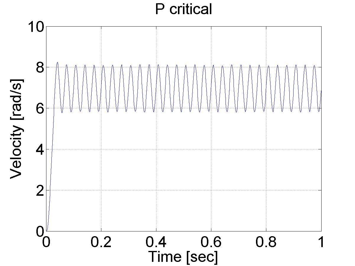
Various controller types are studied next.
In this exercise first P, after PI and at the end PID speed controller is set-up for the DC motor.
Steps:
Study the literature of control theory overviewed in the below chapter entitled “Theoretical background of control theories”.
Set up controller (P, PI, PID, etc.).
Exercise tasks
After studying the basics of P, PI and PID speed control of DC motors, the user can build the controllers for the exercise.
Task 1.
Determine the values for your P, PI and PID controller. This can be done according to Ziegler-Nichols method (see below), by changing the P value until the system starts oscillating. This way the values can be calculated and the controllers can be programmed (please, use low pass filter for the velocity).
Task 2.
Compare the results of the P, and PI controllers for a reference shaft speed Ω = 4 rad/s.
Task 3.
Task 3 is an extension of Task 2, with the difference that in this case we set the reference shaft speed Ω = 4 rad/s at t = 0 s, change it to Ω = 2 rad/s at t = 2 s and again change it Ω = 6 rad/s at t = 4 s.
Task 4.
Compare the P, and PI controllers for disturbance rejection. The disturbance will be applied at t = 0.5 s, as a negative torque T_load= -0.5, which is subtracted from the output voltage calculated by the controller.
ResultData.Torque = (please write here your controller)
ResultData.Torque = ResultData.Torque + T_load; /* this is the line for virtual load*/
Task 5.
Execute the same tasks with open loop and compare the results with those of P, and PI controllers.
The result files, which can be downloaded at the end of the measurement, can be evaluated in Matlab. There is a program already written for this task, which draws the shaft speed-time, voltage-time and position-time diagrams. These diagrams can be saved in jpg formats for further documentation.
Task 6.
Fault tolerance of PI controller (anti-windup PI controller).
Simulate a fault when the motor is blocked or the power electronic unit has a failure and the torque is 0 while the PI controller is operating. The integral term is increasing. After the failure the integral term must be reduced (the integral term of positive error must be compensated by an integral term of negative error).
First tune a PI controller (set the Measurement length to 1000 ms), then add the following line to the controller:
if ( CurrentTime < 0.3*1e3) {ResultData.Torque = 0.0;}
Set different limits for the integral term of PI controller and compare the performances.
Task 7.
Design a sliding mode controller for the position of the motor.
The two main steps of the design of a sliding mode controller are
selection of a proper sliding surface,
selection of a proper control law.
The constant reference position is set to
αref= 10 rad.
The position and speed error are defined as
αe= αref – αmotor
Ωe= 0-Ωmotor .
The sliding surface is selected as
σ=αe+λΩe .
The control law is selected as
torque=0.1 sign σ.
Of course, you have to use C code for the algorithm above. For more detailed information and even newer control theories visit the animation site:
http://dind.mogi.bme.hu/animation/
Chapter 6. Sample measurement
- 6.1. Using the PCI-1720 D/A card -- Exercise 1
- 6.2. Using the real-time clock with PCI 1720 D/A card – Exercise 2
- 6.3. Using the PCI-1784 Counter card -- Exercise 3
- 6.4. Open Loop Control measurement – Motion control/Exercise 4. Open-loop test
- 6.5. Closed Loop Control Measurements -- Exercise 5
- 6.5.1. Parameter tuning of the P controller -- Test 1.
- 6.5.2. Step signal response of the P controller -- Test 2.
- 6.5.3. Response of the P controller to step changes in the reference speed signal -- Test 3.
- 6.5.4. Response of the P controller to step changes in the load -- Test 4.
- 6.5.5. Step signal response of the PI controller -- Test 2.
- 6.5.6. Response of the PI controller to step changes in the reference speed signal -- Test 3.
- 6.5.7. Response of the PI controller to step changes in the load -- Test 4.
- 6.5.8. Step signal response of the P and PI controller -- Test 1.
- 6.5.9. Stick-slip phenomenon
- 6.5.10. Step signal response of the position controller with inner shaft speed controller -- Test 1.
- 6.5.11. Fault tolerance measurements
- 6.5.12. Control of time-delay system
- 6.5.13. Sliding mode control results
- 6.6. Complex design and measurement
- 6.6.1. State feedback and its design
- 6.6.2. Application of reference signal correction
- 6.6.3. Design of the state observer
- 6.6.4. Integral control
- 6.6.5. Identification of the system
- 6.6.6. Design of the control
- 6.6.7. Identification of the motor
- 6.6.8. Design of the control
- 6.6.9. Integral control
- 6.6.10. Filter design for velocity measurement
- 6.6.11. Implementation
- 6.6.12. Control without integrator
- 6.6.13. Results of the measurement
- 6.6.14. Control with the integrator
- 6.6.15. Results of the measurement in the case of integrator
- 6.6.16. Appendix
6.1. Using the PCI-1720 D/A card -- Exercise 1
The code that is the solution and should be pasted into the code box is:
motorDA = 3;
new_voltage = 5.0;
//Step 1: Open device
dwErrCde = DRV_DeviceOpen(lDevNumDA, &lDriverHandleDA);
if (dwErrCde != SUCCESS)
{
    ErrorHandler(dwErrCde);
    exit(1);
}
// Step 2: Output value to the specified channel
tAOVoltageOut.chan = motorDA;
tAOVoltageOut.OutputValue = new_voltage;
dwErrCde = DRV_AOVoltageOut(lDriverHandleDA, &tAOVoltageOut);
if (dwErrCde != SUCCESS)
{
    ErrorStop(&lDriverHandleDA, dwErrCde);
    return;
}
This code turns on the drive unit power. You should see the green LED on the drive unit lit.
To turn off the LED modify the following line: new_voltage = 0.0;
6.1.1. From the sample file (Dasoft.cpp) the following part should be copied to the text box:
//Step 3: Open device
dwErrCde = DRV_DeviceOpen(lDevNum, &lDriverHandle);
if (dwErrCde != SUCCESS)
{
    ErrorHandler(dwErrCde);
    printf("Program terminated!\n");
    printf("Press any key to exit....");
    getch();
    exit(1);
}
// Step 4: Output value to the specified channel
tAOVoltageOut.chan = usChan;
tAOVoltageOut.OutputValue = fOutValue;
dwErrCde = DRV_AOVoltageOut(lDriverHandle, &tAOVoltageOut);
if (dwErrCde != SUCCESS)
{
    ErrorStop(&lDriverHandle, dwErrCde);
    printf("Press any key to exit....");
    getch();
    return;
}
6.1.2. Remove the code parts marked with red.
//Step 3: Open device
dwErrCde = DRV_DeviceOpen(lDevNum, &lDriverHandle);
if (dwErrCde != SUCCESS)
{
    ErrorHandler(dwErrCde);
printf("Program terminated!\n");
    printf("Press any key to exit....");
    getch();
    exit(1);
}
// Step 4: Output value to the specified channel
tAOVoltageOut.chan = usChan;
tAOVoltageOut.OutputValue = fOutValue;
dwErrCde = DRV_AOVoltageOut(lDriverHandle, &tAOVoltageOut);
if (dwErrCde != SUCCESS)
{
    ErrorStop(&lDriverHandle, dwErrCde);
printf("Press any key to exit....");
    getch();
    return;
}
6.1.3. Change the code as it is highlighted with green.
motorDA = 3;
new_voltage = 5.0;
//Step 1: Open device
dwErrCde = DRV_DeviceOpen(lDevNumDA, &lDriverHandleDA);
if (dwErrCde != SUCCESS)
{
    ErrorHandler(dwErrCde);
    exit(1);
}
// Step 2: Output value to the specified channel
tAOVoltageOut.chan = motorDA;
tAOVoltageOut.OutputValue = new_voltage;
dwErrCde = DRV_AOVoltageOut(lDriverHandleDA, &tAOVoltageOut);
if (dwErrCde != SUCCESS)
{
    ErrorStop(&lDriverHandleDA, dwErrCde);
    return;
}
Alternative solution can be achieved without using the predefined variables (motorDA and new_votlage). In this case the code is the following:
//Step 1: Open device
dwErrCde = DRV_DeviceOpen(lDevNumDA, &lDriverHandleDA);
if (dwErrCde != SUCCESS)
{
    ErrorHandler(dwErrCde);
    exit(1);
}
// Step 2: Output value to the specified channel
tAOVoltageOut.chan = 3;
tAOVoltageOut.OutputValue = 5.0f;
dwErrCde = DRV_AOVoltageOut(lDriverHandleDA, &tAOVoltageOut);
if (dwErrCde != SUCCESS)
{
    ErrorStop(&lDriverHandleDA, dwErrCde);
    return;
}
6.2. Using the real-time clock with PCI 1720 D/A card – Exercise 2
The code, which the students should write into the variable box is:
float sin_amp = 3.0;
float sin_ang_freq = 0.25;
The code, which the students should write into the code box is:
new_voltage = sin_amp * sin(sin_ang_freq * (time_array[tickCount] / 10000000.0));
The division of 10000 is needed, to get the milliseconds and 1000 for the seconds.
The sin() function is a built in function of C++ and can be located in the Math.h header file. This function calculates the sinus of the given value.
If you use other variable than new_voltage the program will not work. The result is:
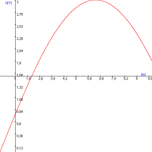
You can directly write in the values, without creating variables for it. In this case the text looks like the following:
new_voltage = 3.0 * sin(0.25 * (time_array[tickCount] / 10000000.0));
6.3. Using the PCI-1784 Counter card -- Exercise 3
The code that is the solution and should be pasted into the first text box (Initialization) is:
//Step 1: Open device
dwErrCde = DRV_DeviceOpen(lDevNumCounter, &lDriverHandleCounter);
if (dwErrCde != SUCCESS)
{
    ErrorHandler(dwErrCde);
    exit(1);
}
// Step 2: Reset counter by DRV_CounterReset
dwErrCde = DRV_CounterReset(lDriverHandleCounter, wChannelCounter);
if (dwErrCde != SUCCESS)
{
    ErrorHandler(dwErrCde);
    exit(1);
}
// Step 3: Start counter operation by DRV_CounterEventStart
tCounterEventStart.counter = wChannelCounter;
dwErrCde = DRV_CounterEventStart(lDriverHandleCounter, &tCounterEventStart);
if (dwErrCde != SUCCESS)
{
    ErrorHandler(dwErrCde);
    exit(1);
}
// Step 4: Read counter value by DRV_CounterEventRead
tCounterEventRead.counter = wChannelCounter;
tCounterEventRead.overflow = &wOverflow;
tCounterEventRead.count = &dwReading;
dwErrCde = DRV_CounterEventRead(lDriverHandleCounter, &tCounterEventRead);
if (dwErrCde != SUCCESS)
{
     ErrorStop(&lDriverHandleCounter, dwErrCde);
     return;
}
The code that is the solution and should be pasted into the second text box (Inside loop) is:
dwErrCde = DRV_CounterEventRead(lDriverHandleCounter, &tCounterEventRead);
if (dwErrCde != SUCCESS)
{
     ErrorStop(&lDriverHandleCounter, dwErrCde);
     return;
}
The results are the position and velocity graphs for a sinus torque.
6.3.1. From the sample file (Dasoft.cpp) the following part should be copied to the text box:
//Step 3: Open device
dwErrCde = DRV_DeviceOpen(lDevNum, &lDriverHandle);
if (dwErrCde != SUCCESS)
{
    ErrorHandler(dwErrCde);
    printf("Program terminated!\n");
    printf("Press any key to exit....");
    getch();
    exit(1);
}
// Step 4: Reset counter by DRV_CounterReset
dwErrCde = DRV_CounterReset(lDriverHandle, wChannel);
if (dwErrCde != SUCCESS)
{
    ErrorHandler(dwErrCde);
    printf("Program terminated!\n");
    printf("Press any key to exit....");
    getch();
    exit(1);
}
// Step 5: Start counter operation by DRV_CounterEventStart
tCounterEventStart.counter = wChannel;
dwErrCde = DRV_CounterEventStart(lDriverHandle, &tCounterEventStart);
if (dwErrCde != SUCCESS)
{
    ErrorHandler(dwErrCde);
    printf("Program terminated!\n");
    printf("Press any key to exit....");
    getch();
    exit(1);
}
// Step 6: Read counter value by DRV_CounterEventRead in while loop
//         and display counter value, exit when pressing any key
tCounterEventRead.counter = wChannel;
tCounterEventRead.overflow = &wOverflow;
tCounterEventRead.count = &dwReading;
while( !kbhit() )
{
   dwErrCde = DRV_CounterEventRead(lDriverHandle, &tCounterEventRead);
   if (dwErrCde != SUCCESS)
   {
      ErrorStop(&lDriverHandle, dwErrCde);
      return;
   }
   printf("\nCounter value = %lu", dwReading);
   Sleep(1000);
}
6.3.2. Remove the code parts marked with red.
//Step 3: Open device
dwErrCde = DRV_DeviceOpen(lDevNum, &lDriverHandle);
if (dwErrCde != SUCCESS)
{
    ErrorHandler(dwErrCde);
printf("Program terminated!\n");
    printf("Press any key to exit....");
    getch();
    exit(1);
}
// Step 4: Reset counter by DRV_CounterReset
dwErrCde = DRV_CounterReset(lDriverHandle, wChannel);
if (dwErrCde != SUCCESS)
{
    ErrorHandler(dwErrCde);
printf("Program terminated!\n");
    printf("Press any key to exit....");
    getch();
    exit(1);
}
// Step 5: Start counter operation by DRV_CounterEventStart
tCounterEventStart.counter = wChannel;
dwErrCde = DRV_CounterEventStart(lDriverHandle, &tCounterEventStart);
if (dwErrCde != SUCCESS)
{
    ErrorHandler(dwErrCde);
printf("Program terminated!\n");
    printf("Press any key to exit....");
    getch();
    exit(1);
}
// Step 6: Read counter value by DRV_CounterEventRead in while loop
//         and display counter value, exit when pressing any key
tCounterEventRead.counter = wChannel;
tCounterEventRead.overflow = &wOverflow;
tCounterEventRead.count = &dwReading;
while( !kbhit() )
{
   dwErrCde = DRV_CounterEventRead(lDriverHandle, &tCounterEventRead);
   if (dwErrCde != SUCCESS)
   {
      ErrorStop(&lDriverHandle, dwErrCde);
      return;
   }
   printf("\nCounter value = %lu", dwReading);
Sleep(1000);
}
6.3.3. Change the code as it is highlighted with green.
//Step 1: Open device
dwErrCde = DRV_DeviceOpen(lDevNumCounter, &lDriverHandleCounter);
if (dwErrCde != SUCCESS)
{
    ErrorHandler(dwErrCde);
    exit(1);
}
// Step 2: Reset counter by DRV_CounterReset
dwErrCde = DRV_CounterReset(lDriverHandleCounter, wChannelCounter);
if (dwErrCde != SUCCESS)
{
    ErrorHandler(dwErrCde);
    exit(1);
}
// Step 3: Start counter operation by DRV_CounterEventStart
tCounterEventStart.counter = wChannelCounter;
dwErrCde = DRV_CounterEventStart(lDriverHandleCounter, &tCounterEventStart);
if (dwErrCde != SUCCESS)
{
    ErrorHandler(dwErrCde);
    exit(1);
}
// Step 4: Read counter value by DRV_CounterEventRead
tCounterEventRead.counter = wChannelCounter;
tCounterEventRead.overflow = &wOverflow;
tCounterEventRead.count = &dwReading;
dwErrCde = DRV_CounterEventRead(lDriverHandleCounter, &tCounterEventRead);
if (dwErrCde != SUCCESS)
{
     ErrorStop(&lDriverHandleCounter, dwErrCde);
     return;
}
Inside loop:
dwErrCde = DRV_CounterEventRead(lDriverHandleCounter, &tCounterEventRead);
if (dwErrCde != SUCCESS)
{
     ErrorStop(&lDriverHandleCounter, dwErrCde);
     return;
}
6.4. Open Loop Control measurement – Motion control/Exercise 4. Open-loop test
For the open loop test, we can do several tests. The output voltage can be calculated from the motor parameters. As there is no feedback in this control, we do not have knowledge about the actual shaft speed of the motor and the disturbance is fully present.
6.4.1. Task 1. Response of the motor to constant torque
The motor was tested with different output torque in this case. 0.1 was applied in the first case and 1 in the second case. The controller has the following form without any declarations:
Measurement length in milliseconds: 1000
The state variable names:
time (given)
position (given)
velocity (given)
torque (given)
Declaration:
Controller:
ResultData.Torque = 1;
or
ResultData.Torque = 0.1;
The results can be seen in the figure bellow. We can see that the position and the shaft speed diagram that the motor has a constant acceleration until it reaches its final shaft speed. The open loop control is very slow because of the constant voltage applied.
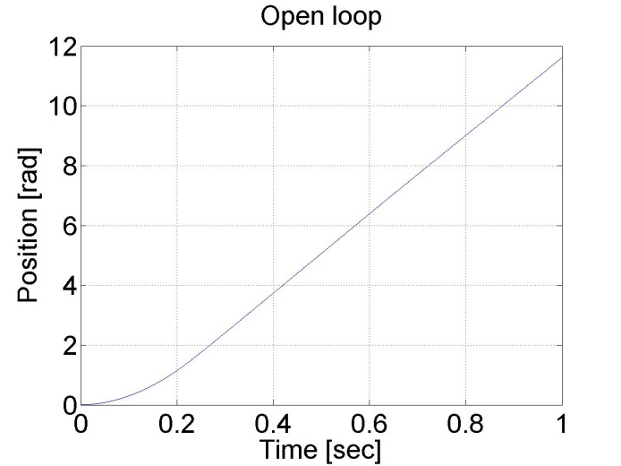

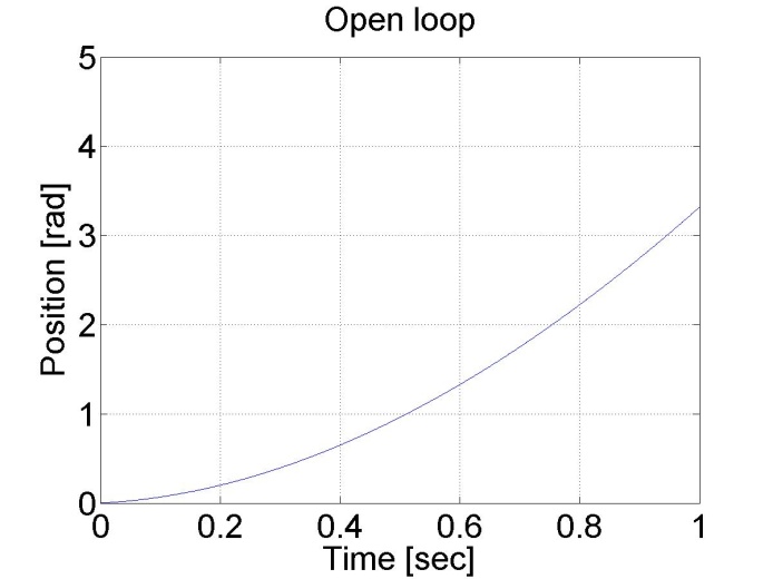
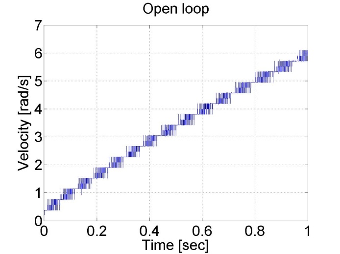
6.4.2. Task 2. Digital filter
The motor was tested with different output torque in this case. In the first case was applied 0.1 and 1 in the second case.
Measurement length in milliseconds: 1000
The state variable names:
time (given)
position (given)
velocity (given)
torque (given)
Declaration:
/* velocity filter variables */
static float  z_1=0.0, z_2=0.0, z_3=0.0;
static float ztmp_1=0.0, ztmp_2=0.0;
/* velocity filter parameters */
/* TSAMPLE=1e-3 and Tc=0.007 */
float ad11= 0.9996, ad12= 9.9072e-004, ad13= 4.3344e-007;
float ad21= -1.2637, ad22= 0.9730, ad23= 8.0496e-004;
float ad31= -2.3468e+003, ad32= -50.5468, ad33= 0.6280;
float bd1= 4.3671e-004, bd2= 1.2637, bd3= 2.3468e+003;
Controller:
/* Velocity filter  */
ztmp_1=ad11* z_1+ad12* z_2+ad13* z_3 + bd1* ResultData.Velocity;
ztmp_2=ad21* z_1+ad22* z_2+ad23* z_3 + bd2* ResultData.Velocity;
z_3=ad31* z_1+ad32* z_2+ad33* z_3 + bd3* ResultData.Velocity;
z_1  = ztmp_1;
z_2  = ztmp_2;
ResultData.Velocity =z_1;
ResultData.Torque = 1;
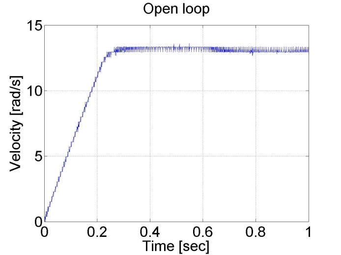
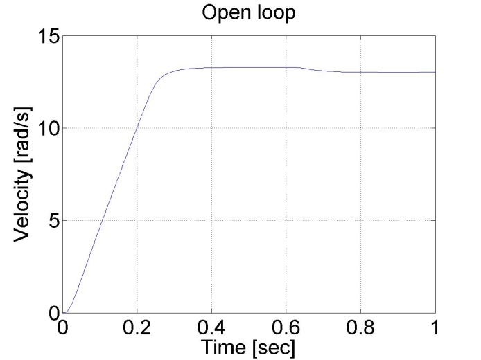
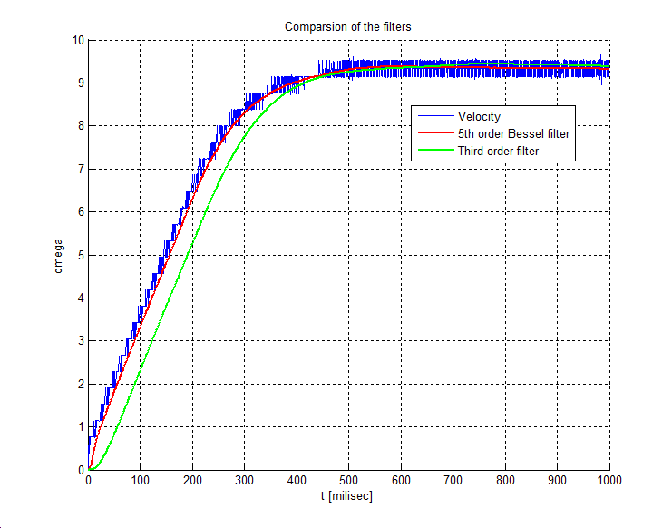
6.4.3. Task 3. Response of the motor to sinusoidal voltage and compensation of the servo amplifier offset
The servo amplifier of has an offset voltage. This is the most obvious if we apply a sinusoidal voltage. In this case we expect the motor to have sinusoidal shaft speed and sinusoidal position change coming from the shaft speed.
Measurement length in milliseconds: 4000
The state variable names:
time (given)
position (given)
velocity (given)
torque (given)
sin_torque (selected)
Declaration:
doubleparam = 0;
doublesinperiod = 1;
doublesinamplitude = 2;
doubleoffset = 0;
// please, change the offset in the range of -0.3 and -0.2
Controller:
// Current time in miliseconds
param = CurrentTime;
// Current time in seconds
param /= 1000;
// Result
param = param * 2 * PI / sinperiod;
//
// Controller part begin
//
// Sinusoidal voltage
ResultData.Torque = sinamplitude * sin(param) + offset;
ResultData.StateVariable_5 = sinamplitude * sin(param);
//
// Controller part end
The results can be seen in the figure bellow. The position diagram is not pure sinusoidal, but it has a linear component too. This linear component is the offset of the servo amplifier. This can be subtracted from the applied voltage and this way the linear component in the position diagram disappears. The only change in the controller is in the declaration:
doubleoffset = -0.27;
The MATLAB program to plot the results
% please, modify it according to you file names
sv_1_14axc255hnyzli55axowlm55
sv_2_14axc255hnyzli55axowlm55
sv_3_14axc255hnyzli55axowlm55
sv_4_14axc255hnyzli55axowlm55
sv_5_14axc255hnyzli55axowlm55
time=time/1000;
plot(time,position)
set(gca, 'fontsize', [25]);
xlabel('Time [sec]');
ylabel('Position [rad]');
title('Open loop');
% you can adjust your axis
axis([0 4 0 12]);
grid
pause;
print -djpeg open_poz
plot(time,velocity)
set(gca, 'fontsize', [25]);
xlabel('Time [sec]');
ylabel('Velocity [rad/s]');
title('Open loop');
% you can adjust your axis
axis([0 4 -15 15]);
grid
print -djpeg open_vel
pause;
plot(time,torque)
set(gca, 'fontsize', [25]);
xlabel('Time [sec]');
ylabel('Torque [mNm]');
title('Open loop');
% you can adjust your axis
axis([0 4 -2.5 2.5]);
grid
print -djpeg open_torque
pause;
plot(time,sin_torque)
set(gca, 'fontsize', [25]);
xlabel('Time [sec]');
ylabel('Torque without offset');
title('Open loop');
% you can adjust your axis
axis([0 4 -2.5 2.5]);
grid
print -djpeg open_sin
|
|
|
|
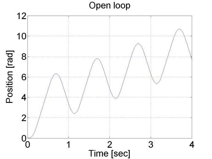
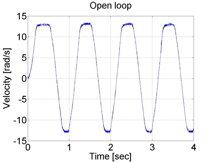
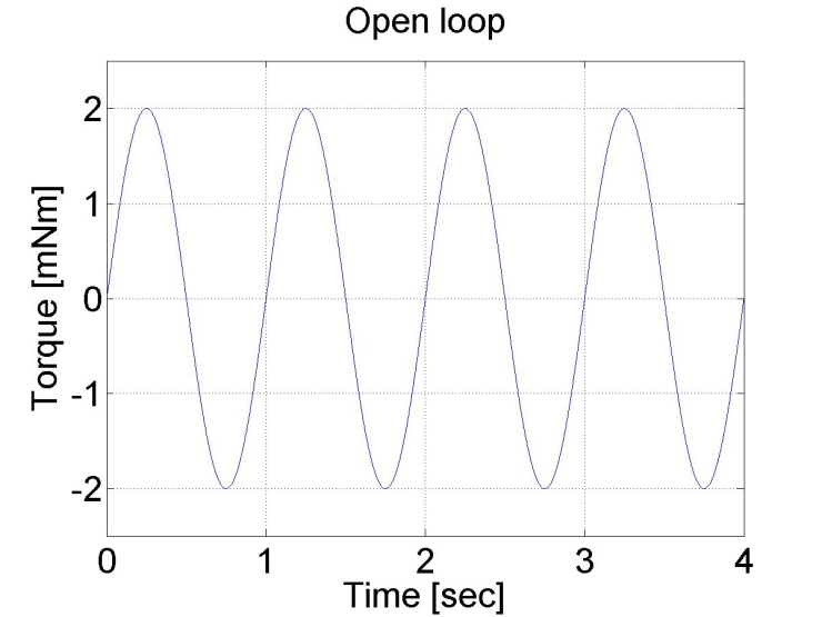

(a)
|
|
|
|
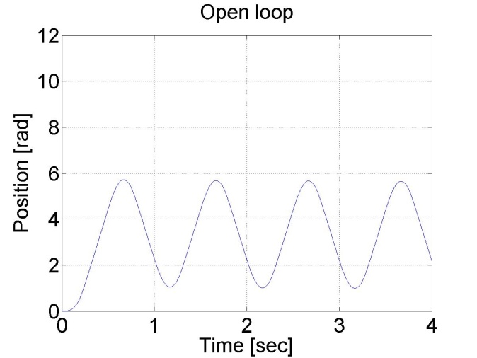
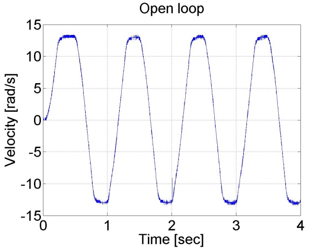
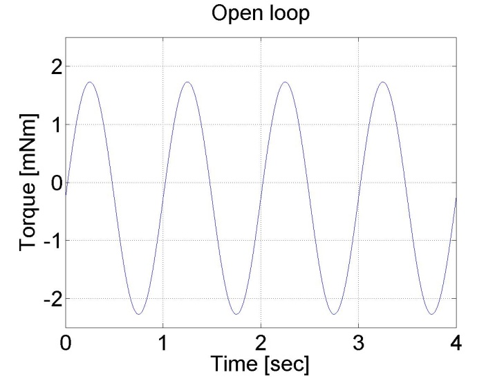
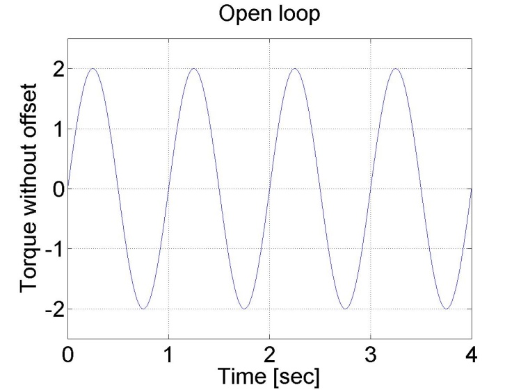
(b)
6.4.4. Comparison of digital filters
Measurement length in milliseconds: 4000
The state variable names:
time (given)
position (given)
velocity (given)
torque (given)
sin_torque (selected)
ref (selected)
filt (selected)
filtb (selected)
Declaration:
doubleparam = 0;
doublesinperiod = 0.1;
doublesinamplitude = 0.6;
doubleoffset = -0.217;
/* variables for filter */
static float  z_1=0.0, z_2=0.0, z_3=0.0;
static float ztmp_1=0.0, ztmp_2=0.0;
/* Tsample=1e-3  Tc=0.0032*/
float ad11 = 0.99591;
float ad12 = 0.00095987;
float ad13 = 3.652e-007;
float ad21 = -11.3235;
float ad22 = 0.88778;
float ad23 = 0.00061567;
float ad31 = -19089.6748;
float ad32 = -193.6165;
float ad33 = 0.30752;
float bd1  = 0.0040906;
float bd2  = 11.3235;
float bd3  = 19089.6748;
/* Variables for Bessel filter */
static float  z_1b=0.0, z_2b=0.0, z_3b=0.0;
static float ztmp_1b=0.0, ztmp_2b=0.0;
/* Bessel Tsample=1e-3  Tc=0.0032*/
float ad11b = 0.95193;
float ad12b = 0.00083371;
float ad13b = 2.6009e-007;
float ad21b = -120.9668;
float ad22b = 0.56688;
float ad23b = 0.00034345;
float ad31b = -159737.83;
float ad32b = -629.4281;
float ad33b = -0.080513;
float bd1b  = 0.048071;
float bd2b  = 120.9668;
float bd3b  = 159737.83;
Controller:
// Current time
param = CurrentTime;
// Only milliseconds
param /= 1000;
// Result
param = param * 2 * PI / sinperiod;
//
// Controller part begin
//
// Sinusoidal voltage
ResultData.Torque = sinamplitude * sin(param) + offset;
ResultData.StateVariable_5 = sinamplitude * sin(param);
/* Velocity filter  */
ztmp_1=ad11* z_1+ad12* z_2+ad13* z_3 + bd1* ResultData.Velocity;
ztmp_2=ad21* z_1+ad22* z_2+ad23* z_3 + bd2* ResultData.Velocity;
z_3=ad31* z_1+ad32* z_2+ad33* z_3 + bd3* ResultData.Velocity;
z_1  = ztmp_1;
z_2  = ztmp_2;
ResultData.StateVariable_6=z_1;
/* Bessel velocity filter  */
ztmp_1b=ad11b* z_1b+ad12b* z_2b+ad13b* z_3b + bd1b* ResultData.Velocity;
ztmp_2b=ad21b* z_1b+ad22b* z_2b+ad23b* z_3b + bd2b* ResultData.Velocity;
z_3b=ad31b* z_1b+ad32b* z_2b+ad33b* z_3b + bd3b* ResultData.Velocity;
z_1b  = ztmp_1b;
z_2b  = ztmp_2b;
ResultData.StateVariable_7=z_1b;
Measurement with two different frequency
doublesinperiod = 0.1;
and
doublesinperiod = 0.5;
The steady state are plotted in Figure 6-1 and Figure 6-2
The MATLAB program for generating Figure 6-1 and Figure 6-2
sv_1_zlwzmf45pqyn1c45p31cvve4
sv_2_zlwzmf45pqyn1c45p31cvve4
sv_3_zlwzmf45pqyn1c45p31cvve4
sv_4_zlwzmf45pqyn1c45p31cvve4
sv_5_zlwzmf45pqyn1c45p31cvve4
sv_6_zlwzmf45pqyn1c45p31cvve4
sv_7_zlwzmf45pqyn1c45p31cvve4

plot(time,velocity,time,filt,time,filtb,time,ref)
set(gca, 'fontsize', [25]);
xlabel('Time [sec]');
ylabel('Velocity [rad/s]');
title('Open loop');
% you can adjust your axis
% axis([0.8 1 -1 1]);
axis([4 5 -3 3]);
grid
print -djpeg open_vel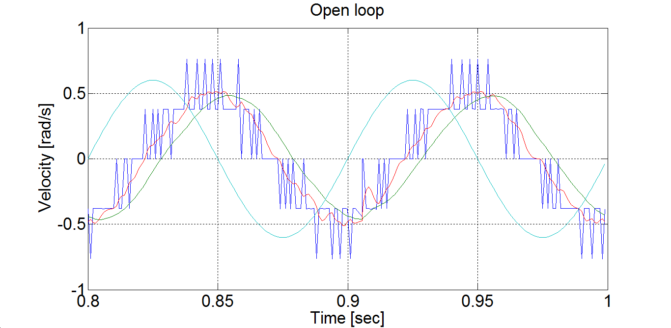
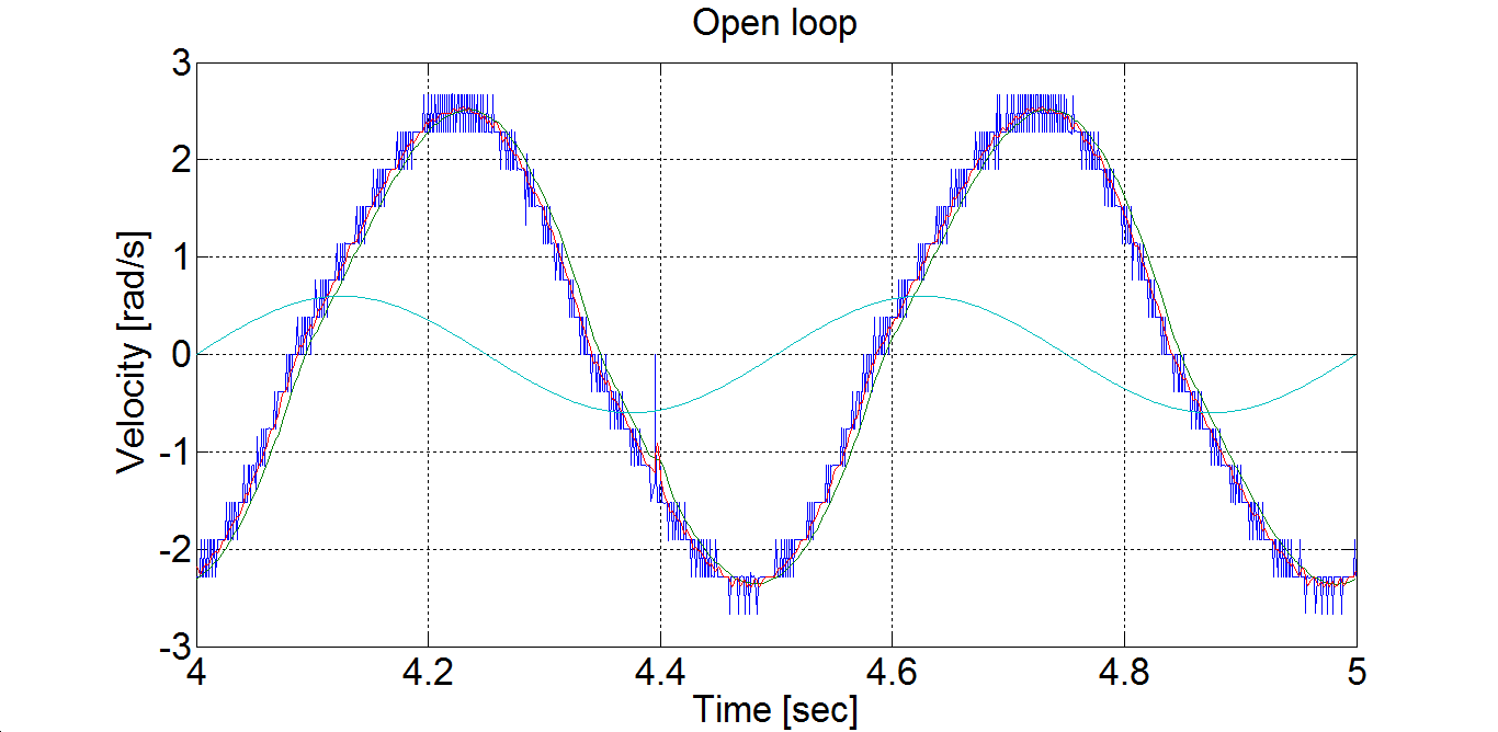
6.5. Closed Loop Control Measurements -- Exercise 5
6.5.1. Parameter tuning of the P controller -- Test 1.
The first task in PID control is to tune the parameters of the controller. For this we used the Ziegler-Nichols method which is easy to implement empirically for the system even for a beginner in control theory. In the figure bellow the Ziegler-Nichols tuning chart can be seen.
AP | I | TD | |
P control | AU/2 | ||
PI control | AU/2.2 | 1.2AP/Tu | |
PID control zó | AU/1.7 | 2AP/Tu | AP Tu/8 |
The first step in the tuning is to create a P controller with arbitrary AU value. The controller has the following form:
Measurement length in milliseconds: 1000
The state variable names:
time (given)
position (given)
velocity (given)
torque (given)
ref (selected)
error (selected)
Declaration:
doubleP = 4.75;
doubleref_vel = 7;
doubleerror_vel= 0;
/* velocity filter variables */
static float  z_1=0.0, z_2=0.0, z_3=0.0;
static float ztmp_1=0.0, ztmp_2=0.0;
/* velocity filter parameters */
/* TSAMPLE=1e-3 and Tc=0.005 */
float ad11= 0.9989, ad12= 9.8248e-004, ad13= 4.0937e-007;
float ad21= -3.2749, ad22= 0.9497, ad23= 7.3686e-004;
float ad31= -5.8949e+003, ad32= -91.6978, ad33= 0.5076;
float bd1= 0.0011, bd2= 3.2749, bd3= 5.8949e+003;
Controller:
/* Velocity filter  */
ztmp_1=ad11* z_1+ad12* z_2+ad13* z_3 + bd1* ResultData.Velocity;
ztmp_2=ad21* z_1+ad22* z_2+ad23* z_3 + bd2* ResultData.Velocity;
z_3=ad31* z_1+ad32* z_2+ad33* z_3 + bd3* ResultData.Velocity;
z_1  = ztmp_1;
z_2  = ztmp_2;
 ResultData.Velocity =z_1;
//Error calculation for velocity control
error_vel=ref_vel- ResultData.Velocity;
ResultData.StateVariable_5 = ref_vel;
ResultData.StateVariable_6 = error_vel;
ResultData.Torque = P*error_vel;
if (ResultData.Torque > 5)
{
ResultData.Torque = 5;
}
if (ResultData.Torque < -5)
{
ResultData.Torque = -5;
}
The controller also sets the minimal and maximal values of the output voltage to 5 and -5 V. The results can be seen in the figure bellow.
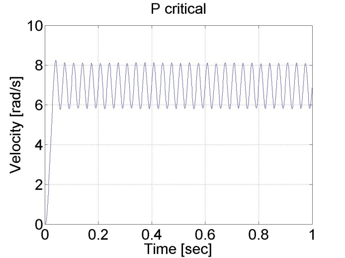
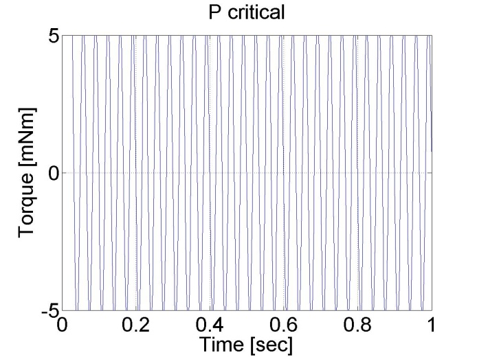
We can conclude that AU = 4.75 and TU≈0.2/6. According to the table PPI=2.1 and IPI=75.
Remark!!! the values of AU and TU depend on the filter parameter.
6.5.2. Step signal response of the P controller -- Test 2.
For this test we set the reference shaft speed to 1 rad/s. The controller has the following form:
Enter measurement length in milliseconds: 1000
The state variable names:
time (given)
position (given)
velocity (given)
torque (given)
ref (selected)
error (selected)
integral (selected)
Declaration:
doubleP_par = 2.3;
doubleI_par = 0.0;
doubleref_vel = 7;
doubleerror_vel;
static doubleerror_vel_int=0.0;
double load = 0;
/* velocity filter variables */
static float z_1=0.0, z_2=0.0, z_3=0.0;
static float ztmp_1=0.0, ztmp_2=0.0;
/* TSAMPLE=1e-3 and Tc=0.0027 */
float ad11= 0.9936, ad12= 9.4621e-004, ad13= 3.4524e-007;
float ad21= - 17.5400, ad22= 0.8515, ad23= 5.6261e-004;
float ad31= -2.8584e+004, ad32= -249.0676, ad33= 0.2264;
float bd1= 0.0064, bd2= 17.5400, bd3= 2.8584e+004;
Controller:
/* Velocity filter */
ztmp_1=ad11* z_1+ad12* z_2+ad13* z_3 + bd1* ResultData.Velocity;
ztmp_2=ad21* z_1+ad22* z_2+ad23* z_3 + bd2* ResultData.Velocity;
z_3=ad31* z_1+ad32* z_2+ad33* z_3 + bd3* ResultData.Velocity;
z_1 = ztmp_1;
z_2 = ztmp_2;
ResultData.Velocity =z_1;
//Error calculation for velocity control
error_vel=ref_vel- ResultData.Velocity;
error_vel_int = error_vel_int + error_vel*(CurrentTime - OldTime)/1000;
ResultData.StateVariable_5 = ref_vel;
ResultData.StateVariable_6 = error_vel;
ResultData.StateVariable_7 = error_vel_int;
ResultData.Torque = P_par*error_vel + I_par*error_vel_int - load;
if (ResultData.Torque > 5) { ResultData.Torque = 5; }
if (ResultData.Torque < -5) { ResultData.Torque = -5; }
The results can be seen in the figure bellow. We can see that the P controller has a constant error in steady state.
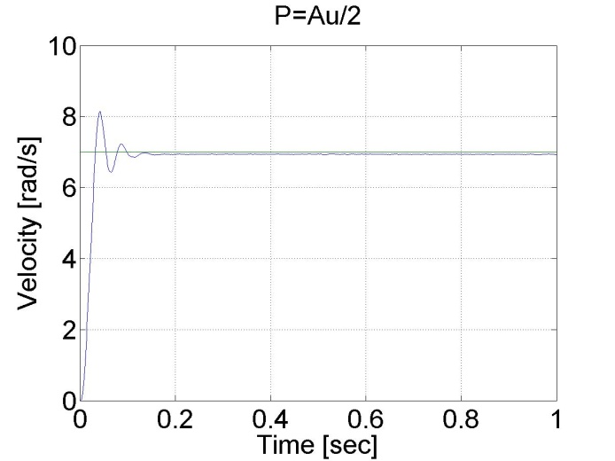
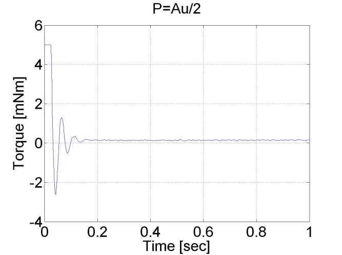
6.5.3. Response of the P controller to step changes in the reference speed signal -- Test 3.
In this test the reference shaft speed changed in two time instances, at t = 0.2 s and at t = 0.4 s. The constant error of the P controller is noticeable in this case too. The controller has the following form:
Enter measurement length in milliseconds: 1000
The state variable names:
time (given)
position (given)
velocity (given)
torque (given)
ref (selected)
error (selected)
integral (selected)
Declaration:
doubleP_par = 2.3;
doubleI_par = 0.0;
doubleref_vel = 7;
doubleerror_vel;
static doubleerror_vel_int=0.0;
double load = 0;
/* velocity filter variables */
static float z_1=0.0, z_2=0.0, z_3=0.0;
static float ztmp_1=0.0, ztmp_2=0.0;
/* TSAMPLE=1e-3 and Tc=0.0027 */
float ad11= 0.9936, ad12= 9.4621e-004, ad13= 3.4524e-007;
float ad21= - 17.5400, ad22= 0.8515, ad23= 5.6261e-004;
float ad31= -2.8584e+004, ad32= -249.0676, ad33= 0.2264;
float bd1= 0.0064, bd2= 17.5400, bd3= 2.8584e+004;
Controller:
//Step changes in reference speed
if (CurrentTime > 0*1e3 && CurrentTime < 0.2*1e3)
{
ref_vel = 4;
}
if (CurrentTime >= 0.2*1e3 && CurrentTime < 0.4*1e3)
{
ref_vel = 8;
}
if (CurrentTime >= 0.4*1e3 && CurrentTime < 0.6*1e3)
{
ref_vel = 2;
}
/* Velocity filter */
ztmp_1=ad11* z_1+ad12* z_2+ad13* z_3 + bd1* ResultData.Velocity;
ztmp_2=ad21* z_1+ad22* z_2+ad23* z_3 + bd2* ResultData.Velocity;
z_3=ad31* z_1+ad32* z_2+ad33* z_3 + bd3* ResultData.Velocity;
z_1 = ztmp_1;
z_2 = ztmp_2;
ResultData.Velocity =z_1;
//Error calculation for velocity control
error_vel=ref_vel- ResultData.Velocity;
error_vel_int = error_vel_int + error_vel*(CurrentTime - OldTime)/1000;
ResultData.StateVariable_5 = ref_vel;
ResultData.StateVariable_6 = error_vel;
ResultData.StateVariable_7 = error_vel_int;
ResultData.Torque = P_par*error_vel + I_par*error_vel_int - load;
if (ResultData.Torque > 5) { ResultData.Torque = 5; }
if (ResultData.Torque < -5) { ResultData.Torque = -5; }
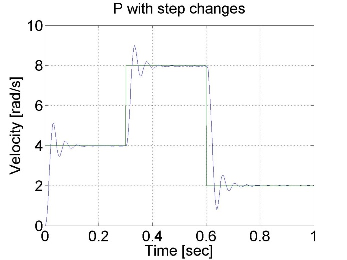
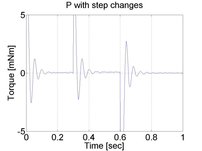
6.5.4. Response of the P controller to step changes in the load -- Test 4.
We can see the largest drawback of the P controller that it has a constant error and it is not able to reject disturbances.
Enter measurement length in milliseconds: 1000
The state variable names:
time (given)
position (given)
velocity (given)
torque (given)
ref (selected)
error (selected)
integral (selected)
Declaration:
doubleP_par = 2.3;
doubleI_par = 0.0;
doubleref_vel = 7;
doubleerror_vel;
static doubleerror_vel_int=0.0;
double load = 2;
/* velocity filter variables */
static float z_1=0.0, z_2=0.0, z_3=0.0;
static float ztmp_1=0.0, ztmp_2=0.0;
/* TSAMPLE=1e-3 and Tc=0.0027 */
float ad11= 0.9936, ad12= 9.4621e-004, ad13= 3.4524e-007;
float ad21= - 17.5400, ad22= 0.8515, ad23= 5.6261e-004;
float ad31= -2.8584e+004, ad32= -249.0676, ad33= 0.2264;
float bd1= 0.0064, bd2= 17.5400, bd3= 2.8584e+004;
Controller:
if (CurrentTime >= 0.4*1e3 && CurrentTime < 0.7*1e3)
{
load = 0.5;
}
/* Velocity filter */
ztmp_1=ad11* z_1+ad12* z_2+ad13* z_3 + bd1* ResultData.Velocity;
ztmp_2=ad21* z_1+ad22* z_2+ad23* z_3 + bd2* ResultData.Velocity;
z_3=ad31* z_1+ad32* z_2+ad33* z_3 + bd3* ResultData.Velocity;
z_1 = ztmp_1;
z_2 = ztmp_2;
ResultData.Velocity =z_1;
//Error calculation for velocity control
error_vel=ref_vel- ResultData.Velocity;
error_vel_int = error_vel_int + error_vel*(CurrentTime - OldTime)/1000;
ResultData.StateVariable_5 = ref_vel;
ResultData.StateVariable_6 = error_vel;
ResultData.StateVariable_7 = error_vel_int;
ResultData.Torque = P_par*error_vel + I_par*error_vel_int - load;
if (ResultData.Torque > 5) { ResultData.Torque = 5; }
if (ResultData.Torque < -5) { ResultData.Torque = -5; }
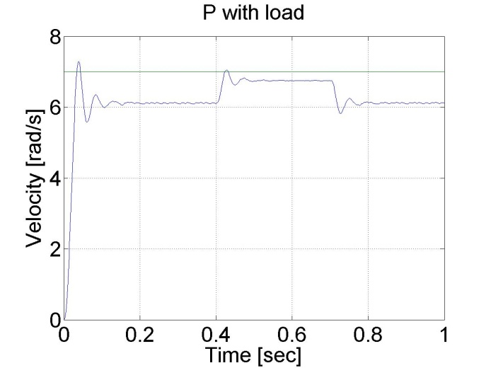
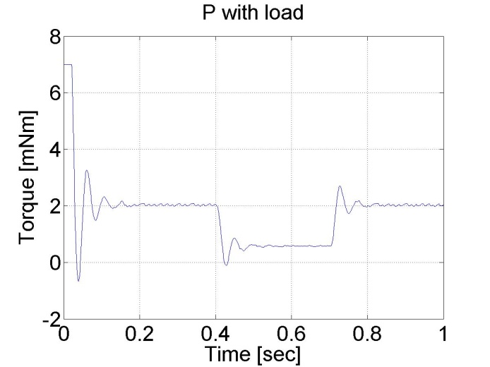
6.5.5. Step signal response of the PI controller -- Test 2.
For this test we set the reference shaft speed to 1 rad/s. The controller has the following form:
Enter measurement length in milliseconds: 1000
The state variable names:
time (given)
position (given)
velocity (given)
torque (given)
ref (selected)
error (selected)
integral (selected)
Declaration:
doubleP = 0.6;
doubleI = 7;
doubleref_vel = 8;
doubleerror_vel;
static doubleerror_vel_int=0.0;
double load = 0;
/* velocity filter variables */
static float z_1=0.0, z_2=0.0, z_3=0.0;
static float ztmp_1=0.0, ztmp_2=0.0;
/* velocity filter parameters */
/* TSAMPLE=1e-3 and Tc=0.007 */
float ad11= 0.9996, ad12= 9.9072e-004, ad13= 4.3344e-007;
float ad21= -1.2637, ad22= 0.9730, ad23= 8.0496e-004;
float ad31= -2.3468e+003, ad32= -50.5468, ad33= 0.6280;
float bd1= 4.3671e-004, bd2= 1.2637, bd3= 2.3468e+003;
Controller:
/* Velocity filter */
ztmp_1=ad11* z_1+ad12* z_2+ad13* z_3 + bd1* ResultData.Velocity;
ztmp_2=ad21* z_1+ad22* z_2+ad23* z_3 + bd2* ResultData.Velocity;
z_3=ad31* z_1+ad32* z_2+ad33* z_3 + bd3* ResultData.Velocity;
z_1 = ztmp_1;
z_2 = ztmp_2;
ResultData.Velocity =z_1;
//Error calculation for velocity control
error_vel=ref_vel- ResultData.Velocity;
error_vel_int = error_vel_int + error_vel*(CurrentTime - OldTime)/1000.0;
ResultData.StateVariable_5 = ref_vel;
ResultData.StateVariable_6 = error_vel;
ResultData.StateVariable_7 = error_vel_int;
ResultData.StateVariable_8 = CurrentTime;
ResultData.Torque = P*error_vel + I*error_vel_int - load;
if (ResultData.Torque > 5)
{
ResultData.Torque = 5;
}
if (ResultData.Torque < -5)
{
ResultData.Torque = -5;
}
The noticeable difference from the P controller is the lack of steady state error. This is the effect of the integral part of the controller, which summarizes the error. The integral error is also presented, which has a large value at the beginning and decreases afterwards. The PI controller is also faster form the P controller. Its drawback is, that is can lead to large overshot or even to instability. This can be eliminated by adding a D element to the controller.
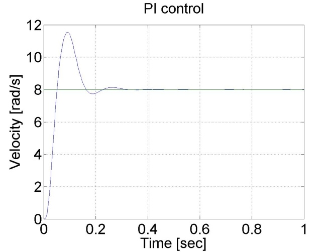
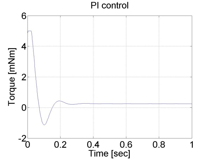
6.5.6. Response of the PI controller to step changes in the reference speed signal -- Test 3.
In this test the reference shaft speed changed in two time instances, at t = 0.3 s and at t = 0.6 s. The PI controller is faster compared to the P controller and the motor operates without steady state error. The controller has the following form:
Enter measurement length in milliseconds: 1000
The state variable names:
time (given)
position (given)
velocity (given)
torque (given)
ref (selected)
error (selected)
integral (selected)
Declaration:
doubleP_par = 2;
doubleI_par = 50.0;
doubleref_vel = 7;
doubleerror_vel;
static doubleerror_vel_int=0.0;
double load = 0;
/* velocity filter variables */
static float z_1=0.0, z_2=0.0, z_3=0.0;
static float ztmp_1=0.0, ztmp_2=0.0;
/* TSAMPLE=1e-3 and Tc=0.0027 */
float ad11= 0.9936, ad12= 9.4621e-004, ad13= 3.4524e-007;
float ad21= - 17.5400, ad22= 0.8515, ad23= 5.6261e-004;
float ad31= -2.8584e+004, ad32= -249.0676, ad33= 0.2264;
float bd1= 0.0064, bd2= 17.5400, bd3= 2.8584e+004;
Controller:
//Step changes in reference speed
if (CurrentTime > 0*1e3 && CurrentTime < 0.3*1e3)
{
ref_vel = 4;
}
if (CurrentTime >= 0.3*1e3 && CurrentTime < 0.6*1e3)
{
ref_vel = 8;
}
if (CurrentTime >= 0.6*1e3 && CurrentTime < 1.6*1e3)
{
ref_vel = 2;
}
/* Velocity filter */
ztmp_1=ad11* z_1+ad12* z_2+ad13* z_3 + bd1* ResultData.Velocity;
ztmp_2=ad21* z_1+ad22* z_2+ad23* z_3 + bd2* ResultData.Velocity;
z_3=ad31* z_1+ad32* z_2+ad33* z_3 + bd3* ResultData.Velocity;
z_1 = ztmp_1;
z_2 = ztmp_2;
ResultData.Velocity =z_1;
//Error calculation for velocity control
error_vel=ref_vel- ResultData.Velocity;
error_vel_int = error_vel_int + error_vel*(CurrentTime - OldTime)/1000;
ResultData.StateVariable_5 = ref_vel;
ResultData.StateVariable_6 = error_vel;
ResultData.StateVariable_7 = error_vel_int;
ResultData.Torque = P_par*error_vel + I_par*error_vel_int - load;
if (ResultData.Torque > 5) { ResultData.Torque = 5; }
if (ResultData.Torque < -5) { ResultData.Torque = -5; }
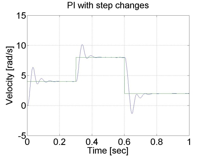
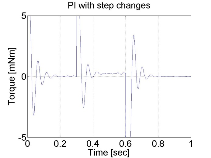
6.5.7. Response of the PI controller to step changes in the load -- Test 4.
In this test, a constant virtual load is added if t < 0.3 s than load=2.0 load, if 0.3 s<t < 0.7 s than load=0.5 finally if t >0.7 s than load=2.0 again.
Enter measurement length in milliseconds: 1000
The state variable names:
time (given)
position (given)
velocity (given)
torque (given)
ref (selected)
error (selected)
integral (selected)
Declaration:
doubleP_par = 2.3;
doubleI_par = 50;
doubleref_vel = 7;
doubleerror_vel;
static doubleerror_vel_int=0.0;
double load = 2;
/* velocity filter variables */
static float z_1=0.0, z_2=0.0, z_3=0.0;
static float ztmp_1=0.0, ztmp_2=0.0;
/* TSAMPLE=1e-3 and Tc=0.0027 */
float ad11= 0.9936, ad12= 9.4621e-004, ad13= 3.4524e-007;
float ad21= - 17.5400, ad22= 0.8515, ad23= 5.6261e-004;
float ad31= -2.8584e+004, ad32= -249.0676, ad33= 0.2264;
float bd1= 0.0064, bd2= 17.5400, bd3= 2.8584e+004;
Controller:
/* Velocity filter */
ztmp_1=ad11* z_1+ad12* z_2+ad13* z_3 + bd1* ResultData.Velocity;
ztmp_2=ad21* z_1+ad22* z_2+ad23* z_3 + bd2* ResultData.Velocity;
z_3=ad31* z_1+ad32* z_2+ad33* z_3 + bd3* ResultData.Velocity;
z_1 = ztmp_1;
z_2 = ztmp_2;
ResultData.Velocity =z_1;
if (CurrentTime >= 0.4*1e3 && CurrentTime < 0.7*1e3)
{
load = 0.5;
}
//Error calculation for velocity control
error_vel=ref_vel- ResultData.Velocity;
error_vel_int = error_vel_int + error_vel*(CurrentTime - OldTime)/1000.0;
ResultData.StateVariable_5 = ref_vel;
ResultData.StateVariable_6 = error_vel;
ResultData.StateVariable_7 = error_vel_int;
ResultData.Torque = P_par*error_vel + I_par*error_vel_int - load;
if (ResultData.Torque > 5)
{
ResultData.Torque = 5;
}
if (ResultData.Torque < -5)
{
ResultData.Torque = -5;
}
We can notice that the PI controller is good at disturbance rejection on the contrary to the P controller.
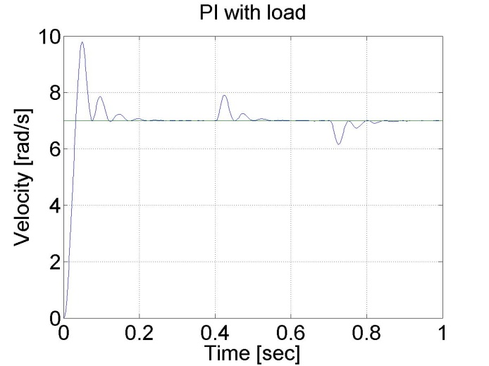
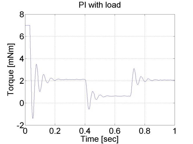
6.5.8. Step signal response of the P and PI controller -- Test 1.
For this test we set the reference shaft position to 10 rad. The controller has the following form:
Enter measurement length in milliseconds: 1000
The state variable names:
time (given)
position (given)
velocity (given)
torque (given)
ref (selected)
error (selected)
integral (selected)
Declaration:
doubleP_par = 1;
doubleI_par = 0;
doubleref_pos = 10;
doubleerror_pos;
static doubleerror_pos_int=0.0;
double load = 0;
/* velocity filter variables */
static float z_1=0.0, z_2=0.0, z_3=0.0;
static float ztmp_1=0.0, ztmp_2=0.0;
/* TSAMPLE=1e-3 and Tc=0.0027 */
float ad11= 0.9936, ad12= 9.4621e-004, ad13= 3.4524e-007;
float ad21= - 17.5400, ad22= 0.8515, ad23= 5.6261e-004;
float ad31= -2.8584e+004, ad32= -249.0676, ad33= 0.2264;
float bd1= 0.0064, bd2= 17.5400, bd3= 2.8584e+004;
static double ini_0 = 0;
static double ini_1 = -10;
Controller:
if (ini_1 < 0)
{
ini_0 = ResultData.Position;
}
ini_1 = 5;
/* Velocity filter */
ztmp_1=ad11* z_1+ad12* z_2+ad13* z_3 + bd1* ResultData.Velocity;
ztmp_2=ad21* z_1+ad22* z_2+ad23* z_3 + bd2* ResultData.Velocity;
z_3=ad31* z_1+ad32* z_2+ad33* z_3 + bd3* ResultData.Velocity;
z_1 = ztmp_1;
z_2 = ztmp_2;
ResultData.Velocity =z_1;
//Error calculation for velocity control
error_pos=ref_pos- ResultData.Position + ini_0;
error_pos_int = error_pos_int + error_pos*(CurrentTime - OldTime)/1000.0;
ResultData.StateVariable_5 = ref_pos;
ResultData.StateVariable_6 = error_pos;
ResultData.StateVariable_7 = error_pos_int;
ResultData.StateVariable_8 = ResultData.Position - ini_0;
ResultData.Torque = P_par*error_pos + I_par*error_pos_int - load;
if (ResultData.Torque > 5)
{
ResultData.Torque = 5;
}
if (ResultData.Torque < -5)
{
ResultData.Torque = -5;
}
We can see that there is a large overshot in this controller, and the steady state error is also present. On the other hand, the position is measured and not calculated by derivation, the position curve is smooth compared to the shaft speed curves in the previous cases.
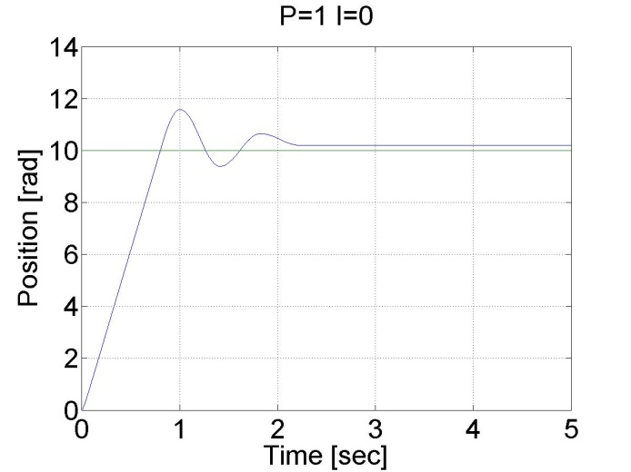
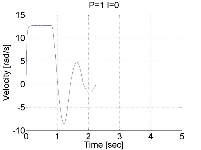
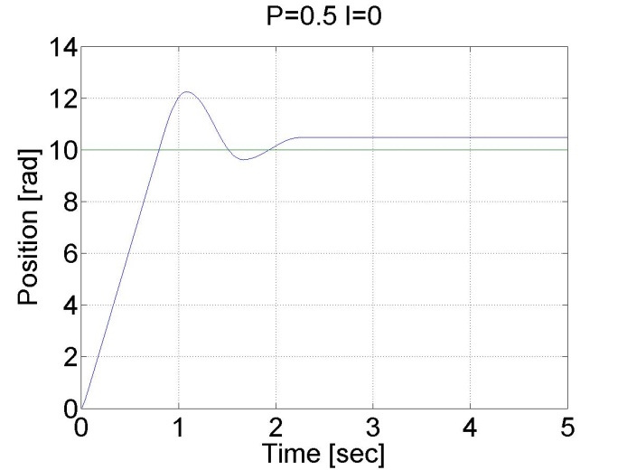
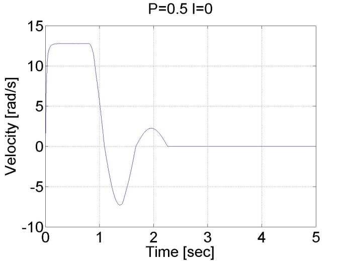
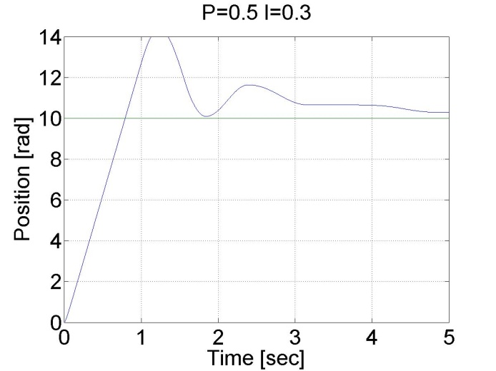
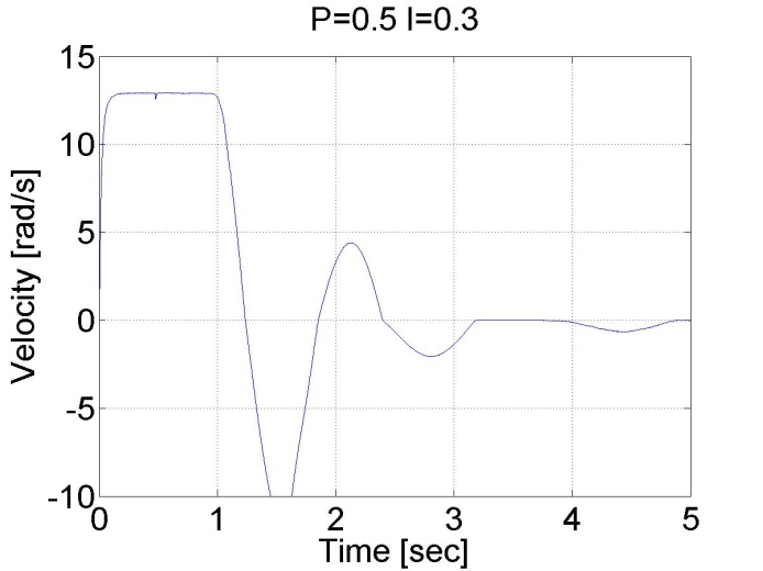
6.5.9. Stick-slip phenomenon
Enter measurement length in milliseconds: 10000
The state variable names:
time (given)
position (given)
velocity (given)
torque (given)
ref (selected)
error (selected)
integral (selected)
Declaration:
doubleP_par = 0.1;
doubleI_par = 0.1;
doubleref_pos = 5;
doubleerror_pos;
static doubleerror_pos_int=0.0;
double load = 0;
/* velocity filter variables */
static float z_1=0.0, z_2=0.0, z_3=0.0;
static float ztmp_1=0.0, ztmp_2=0.0;
/* TSAMPLE=1e-3 and Tc=0.0027 */
float ad11= 0.9936, ad12= 9.4621e-004, ad13= 3.4524e-007;
float ad21= - 17.5400, ad22= 0.8515, ad23= 5.6261e-004;
float ad31= -2.8584e+004, ad32= -249.0676, ad33= 0.2264;
float bd1= 0.0064, bd2= 17.5400, bd3= 2.8584e+004;
static double ini_0 = 0;
static double ini_1 = -10;
Controller:
if (ini_1 < 0)
{
ini_0 = ResultData.Position;
}
ini_1 = 5;
/* Velocity filter */
ztmp_1=ad11* z_1+ad12* z_2+ad13* z_3 + bd1* ResultData.Velocity;
ztmp_2=ad21* z_1+ad22* z_2+ad23* z_3 + bd2* ResultData.Velocity;
z_3=ad31* z_1+ad32* z_2+ad33* z_3 + bd3* ResultData.Velocity;
z_1 = ztmp_1;
z_2 = ztmp_2;
ResultData.Velocity =z_1;
//Error calculation for velocity control
error_pos=ref_pos- CurrentPosition;
error_pos_int = error_pos_int + error_pos*(CurrentTime - OldTime)/1000.0;
ResultData.StateVariable_5 = ref_pos;
ResultData.StateVariable_6 = error_pos;
ResultData.StateVariable_7 = error_pos_int;
ResultData.Torque = P_par*error_pos + I_par*error_pos_int - load;
if (ResultData.Torque > 5)
{
ResultData.Torque = 5;
}
if (ResultData.Torque < -5)
{
ResultData.Torque = -5;
}
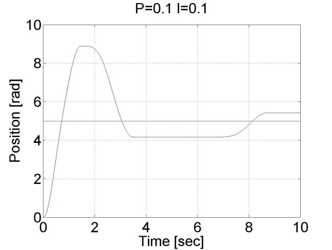
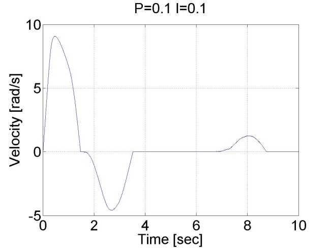
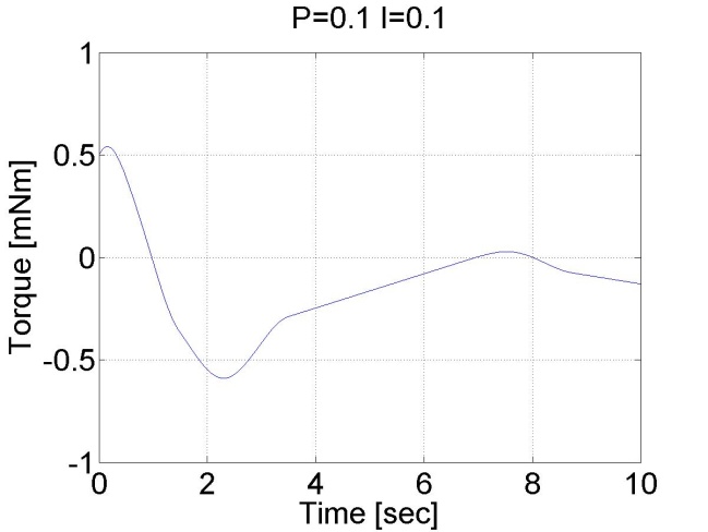
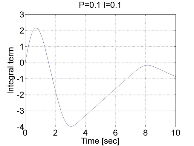
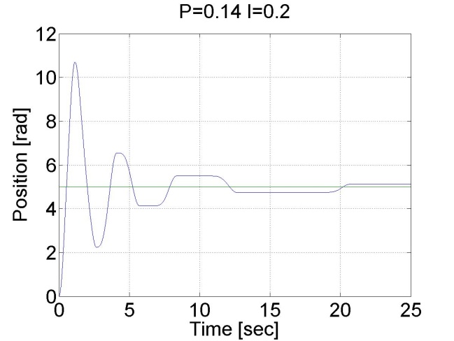
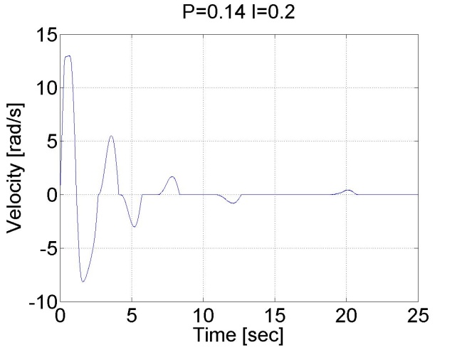
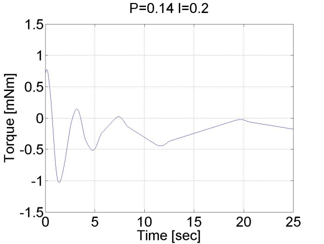
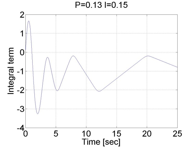
6.5.10. Step signal response of the position controller with inner shaft speed controller -- Test 1.
The motor reached the reference position. The reason for the overshot is that it takes time to decelerate the motor. This effect can be eliminated if we introduce an inner control loop for the shaft speed of the motor. The reference value for the shaft speed is coming from the position error of the motor, this means that as the motor reaches its reference position the reference shaft speed starts do decrease. The reference shaft speed is almost zero if the motor is close to the reference position. The structure of this controller can be seen in the figure bellow. The position controller is P type and the shaft speed controller is PI type.
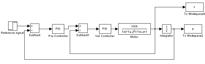
The controller code is the following:
The state variable names:
time (given)
position (given)
velocity (given)
torque (given)
ref_poz (selected)
ref_vel (selected)
err_pos (selected)
err_vel (selected)
int_vel (selected)
poz (selected)
Declaration:
doubleP_pos = 3;
doubleP_vel = 3;
doubleI_vel = 30;
doubleref_pos = 10;
doubleref_vel = 0;
doubleerror_pos = 0;
doubleerror_vel = 0;
static doubleerror_vel_int = 0;
static doubleini_0 = 0;
static doubleini_1 = -10;
/* velocity filter variables */
static float z_1=0.0, z_2=0.0, z_3=0.0;
static float ztmp_1=0.0, ztmp_2=0.0;
/* TSAMPLE=1e-3 and Tc=0.0027 */
float ad11= 0.9936, ad12= 9.4621e-004, ad13= 3.4524e-007;
float ad21= - 17.5400, ad22= 0.8515, ad23= 5.6261e-004;
float ad31= -2.8584e+004, ad32= -249.0676, ad33= 0.2264;
float bd1= 0.0064, bd2= 17.5400, bd3= 2.8584e+004;
Controller:
if (ini_1 < 0)
{
ini_0 = ResultData.Position;
}
ini_1 = 5;
/* Velocity filter */
ztmp_1=ad11* z_1+ad12* z_2+ad13* z_3 + bd1* ResultData.Velocity;
ztmp_2=ad21* z_1+ad22* z_2+ad23* z_3 + bd2* ResultData.Velocity;
z_3=ad31* z_1+ad32* z_2+ad33* z_3 + bd3* ResultData.Velocity;
z_1 = ztmp_1;
z_2 = ztmp_2;
ResultData.Velocity =z_1;
//Error calculation for position control
error_pos = ref_pos- ResultData.Position + ini_0;
// Error calculation for velocity control
ref_vel = error_pos*P_pos;
error_vel = ref_vel - ResultData.Velocity;
error_vel_int = error_vel_int + error_vel*(CurrentTime - OldTime)/1000;
ResultData.StateVariable_5 = ref_pos;
ResultData.StateVariable_6 = ref_vel;
ResultData.StateVariable_7 = error_pos;
ResultData.StateVariable_8 = error_vel;
ResultData.StateVariable_9 = error_vel_int;
ResultData.StateVariable_10 = ResultData.Position - ini_0;
//Controller
ResultData.Torque = P_vel*error_vel + I_vel*error_vel_int;
if (ResultData.Torque > 5)
{
ResultData.Torque = 5;
}
if (ResultData.Torque < -5)
{
ResultData.Torque = -5;
}
We can see that there is no overshot in this case, because the shaft speed starts decreasing in time. We can conclude that position control with inner shaft speed control loop gives much better results than the simple P position controller.

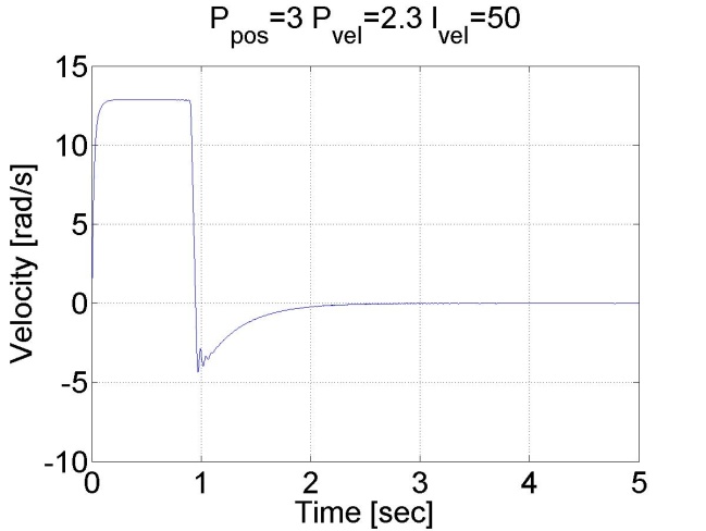
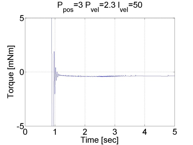
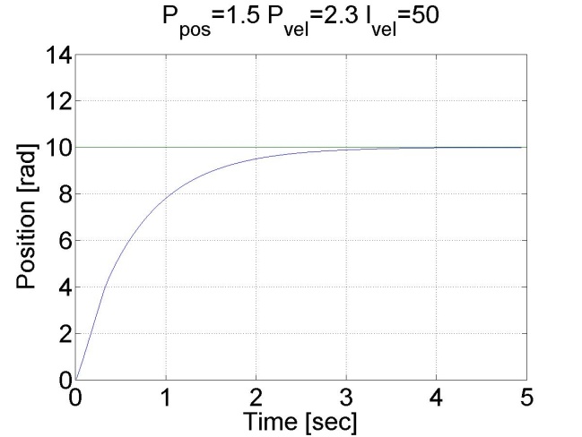
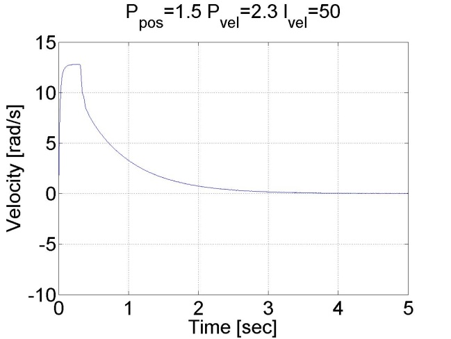
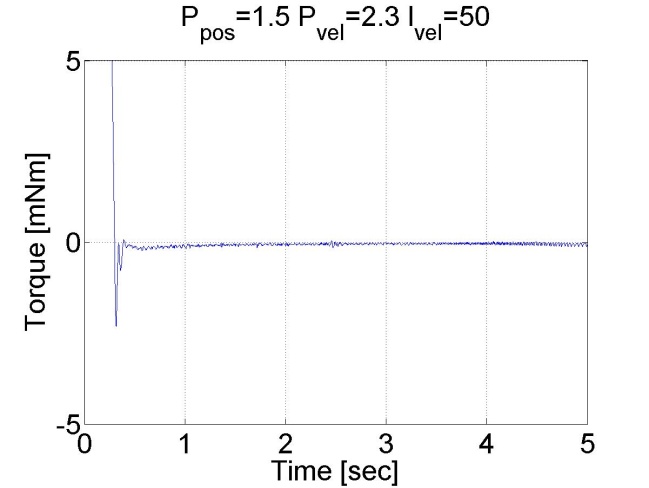

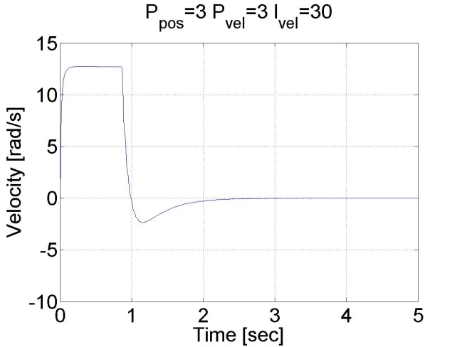
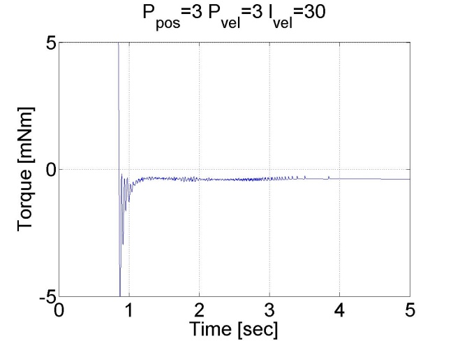
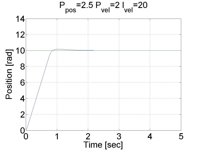
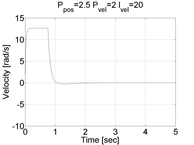
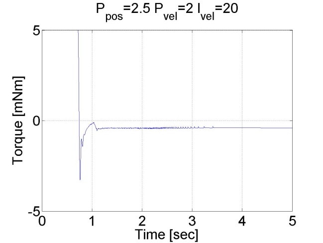
6.5.11. Fault tolerance measurements
Enter measurement length in milliseconds: 1000
The state variable names:
time (given)
position (given)
velocity (given)
torque (given)
ref (selected)
error (selected)
integral (selected)
Declaration:
doubleP_par = 2;
doubleI_par = 50;
doubleref_vel = 7;
doubleerror_vel;
static doubleerror_vel_int=0.0;
double load = 0;
/*
// in case of a
doubleint_lim = 100;
doubleTf = -0.3*1e3;
// in case of b
doubleint_lim = 100;
doubleTf = 0.3*1e3;
// in case of c
doubleint_lim = 0.9;
doubleTf = 0.3*1e3;
// in case of d
doubleint_lim = 0.15;
doubleTf = 0.3*1e3;
*/
// Please, copy one of the above pair of parameters
doubleint_lim = 0.15;
doubleTf = 0.3*1e3;
Controller:
/* velocity filter variables */
static float z_1=0.0, z_2=0.0, z_3=0.0;
static float ztmp_1=0.0, ztmp_2=0.0;
/* TSAMPLE=1e-3 and Tc=0.0027 */
float ad11= 0.9936, ad12= 9.4621e-004, ad13= 3.4524e-007;
float ad21= - 17.5400, ad22= 0.8515, ad23= 5.6261e-004;
float ad31= -2.8584e+004, ad32= -249.0676, ad33= 0.2264;
float bd1= 0.0064, bd2= 17.5400, bd3= 2.8584e+004;
/* Velocity filter */
ztmp_1=ad11* z_1+ad12* z_2+ad13* z_3 + bd1* ResultData.Velocity;
ztmp_2=ad21* z_1+ad22* z_2+ad23* z_3 + bd2* ResultData.Velocity;
z_3=ad31* z_1+ad32* z_2+ad33* z_3 + bd3* ResultData.Velocity;
z_1 = ztmp_1;
z_2 = ztmp_2;
ResultData.Velocity =z_1;
//Error calculation for velocity control
error_vel=ref_vel- ResultData.Velocity;
error_vel_int = error_vel_int + error_vel*(CurrentTime - OldTime)/1000.0;
ResultData.StateVariable_5 = ref_vel;
ResultData.StateVariable_6 = error_vel;
ResultData.StateVariable_7 = error_vel_int;
if (error_vel_int > int_lim)
{
error_vel_int = int_lim;
}
ResultData.Torque = P_par*error_vel + I_par*error_vel_int - load;
if ( CurrentTime < Tf)
{
ResultData.Torque = 0.0;
}
if (ResultData.Torque > 5)
{
ResultData.Torque = 5;
}
if (ResultData.Torque < -5)
{
ResultData.Torque = -5;
}
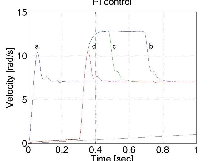
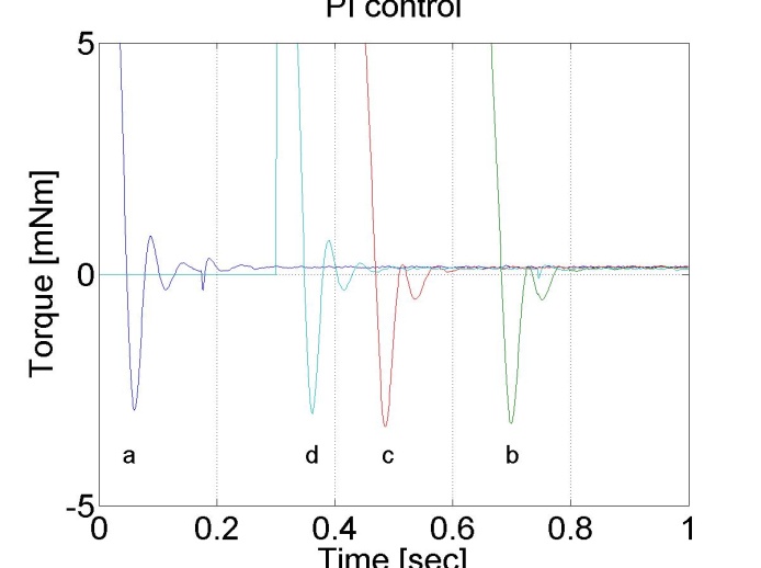
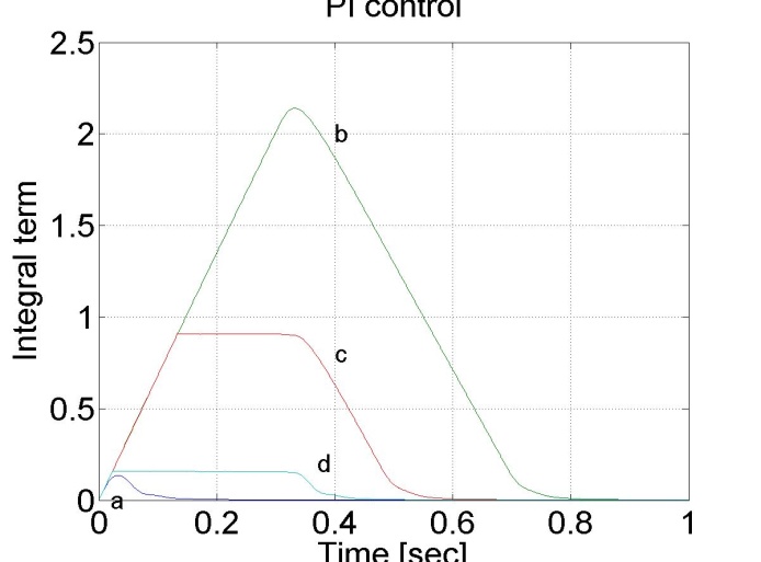
Enter measurement length in milliseconds: 1000
The state variable names:
time (given)
position (given)
velocity (given)
torque (given)
ref (selected)
error (selected)
integral (selected)
Declaration:
doubleP_par = 2.1;
doubleI_par = 75.0;
doubleref_vel = 7;
doubleerror_vel;
static doubleerror_vel_int=0.0;
double load = 2;
double delta = 0;
/* velocity filter variables */
static float z_1=0.0, z_2=0.0, z_3=0.0;
static float ztmp_1=0.0, ztmp_2=0.0;
/* Tsample=1e-3 and Tc=0.0027 */
float ad11= 0.9936, ad12= 9.4621e-004, ad13= 3.4524e-007;
float ad21= - 17.5400, ad22= 0.8515, ad23= 5.6261e-004;
float ad31= -2.8584e+004, ad32= -249.0676, ad33= 0.2264;
float bd1= 0.0064, bd2= 17.5400, bd3= 2.8584e+004;
Controller:
/* Velocity filter */
ztmp_1=ad11* z_1+ad12* z_2+ad13* z_3 + bd1* ResultData.Velocity;
ztmp_2=ad21* z_1+ad22* z_2+ad23* z_3 + bd2* ResultData.Velocity;
z_3=ad31* z_1+ad32* z_2+ad33* z_3 + bd3* ResultData.Velocity;
z_1 = ztmp_1;
z_2 = ztmp_2;
ResultData.Velocity =z_1;
//Error calculation for velocity control
error_vel=ref_vel- ResultData.Velocity;
delta=error_vel*(CurrentTime - OldTime)/1000;
error_vel_int = error_vel_int + delta;
ResultData.StateVariable_5 = ref_vel;
ResultData.StateVariable_6 = error_vel;
ResultData.Torque = P_par*error_vel + I_par*error_vel_int - load;
if (ResultData.Torque > 5) { ResultData.Torque = 5; error_vel_int = error_vel_int - delta*0; }
if (ResultData.Torque < -5) { ResultData.Torque = -5; error_vel_int = error_vel_int - delta*0;}
ResultData.StateVariable_7 = error_vel_int;
The oveshoot can be reduced by switching off the integrator term during controller saturation
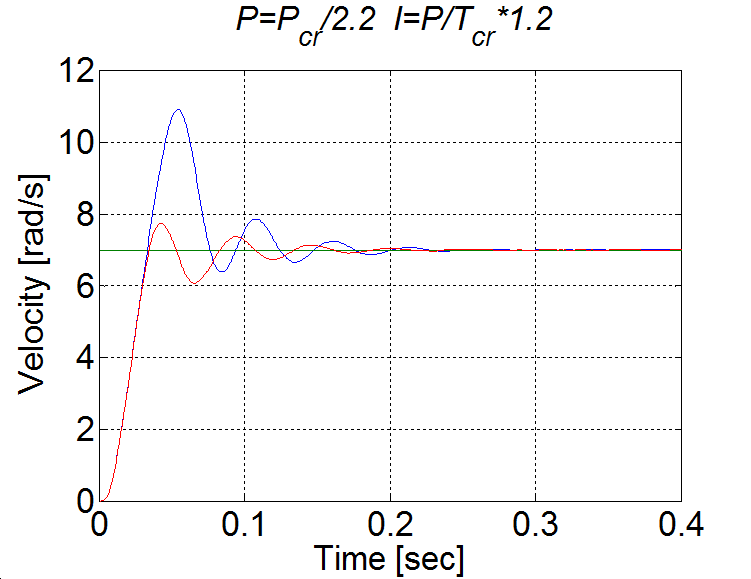
Comparision of the integral terms in two cases
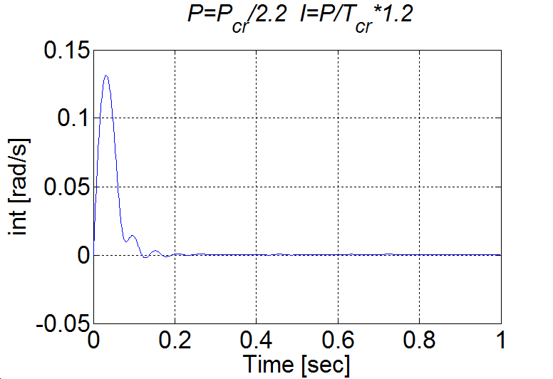
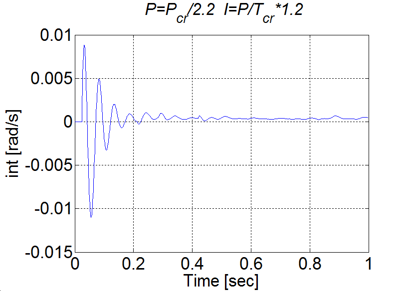
6.5.12. Control of time-delay system
Enter measurement length in milliseconds: 1000
The state variable names:
time (given)
position (given)
velocity (given)
torque (given)
ref (selected)
error (selected)
integral (selected)
Declaration:
doubleP_par = 0.85;
doubleI_par = 12.0;
doubleref_vel = 7;
doubleerror_vel;
static doubleerror_vel_int=0.0;
double load = 0;
/* Time delay pipe */
static float T_1=0.0, T_2=0.0, T_3=0.0;
static float T_4=0.0, T_5=0.0, T_6=0.0;
static float T_7=0.0, T_8=0.0, T_9=0.0;
/* velocity filter variables */
static float z_1=0.0, z_2=0.0, z_3=0.0;
static float ztmp_1=0.0, ztmp_2=0.0;
/* Tsample=1e-3 and Tc=0.0032 */
float ad11 = 0.99591, ad12 = 0.00095987, ad13 = 3.652e-007;
float ad21 = -11.3235, ad22 = 0.88778, ad23 = 0.00061567;
float ad31 = -19089.6748, ad32 = -193.6165, ad33 = 0.30752;
float bd1 = 0.0040906, bd2 = 11.3235, bd3 = 19089.6748;
Controller:
//Step changes in reference speed
/* Velocity filter */
ztmp_1=ad11* z_1+ad12* z_2+ad13* z_3 + bd1* ResultData.Velocity;
ztmp_2=ad21* z_1+ad22* z_2+ad23* z_3 + bd2* ResultData.Velocity;
z_3=ad31* z_1+ad32* z_2+ad33* z_3 + bd3* ResultData.Velocity;
z_1 = ztmp_1;
z_2 = ztmp_2;
ResultData.Velocity =z_1;
//Error calculation for velocity control
error_vel=ref_vel- ResultData.Velocity;
error_vel_int = error_vel_int + error_vel*(CurrentTime - OldTime)/1000;
ResultData.StateVariable_5 = ref_vel;
ResultData.StateVariable_6 = error_vel;
ResultData.StateVariable_7 = error_vel_int;
ResultData.Torque = T_1;
T_1=T_2;
T_2=T_3;
T_3=T_4;
T_4=T_5;
T_5=T_6;
T_6=T_7;
T_7=T_8;
T_8=T_9;
T_9= P_par*error_vel + I_par*error_vel_int - load;
if (T_9 > 5) { T_9 = 5;
error_vel_int = error_vel_int - error_vel*(CurrentTime - OldTime)/1000;}
if (T_9 < -5) { T_9 = -5;
error_vel_int = error_vel_int - error_vel*(CurrentTime - OldTime)/1000;}
Az eredményeket megjelenítő MATLAB program
% please, modify it according to you file names
sv_1_hwztupv131qjbi55l3k5oi45
sv_2_hwztupv131qjbi55l3k5oi45
sv_3_hwztupv131qjbi55l3k5oi45
sv_4_hwztupv131qjbi55l3k5oi45
sv_5_hwztupv131qjbi55l3k5oi45
sv_6_hwztupv131qjbi55l3k5oi45
sv_7_hwztupv131qjbi55l3k5oi45
time=time/1000;
plot(time,position)
set(gca, 'fontsize', [25]);
xlabel('Time [sec]');
ylabel('Position [rad]');
title('Delyed system with PI controller');
% you can adjust your axis
axis([0 1 0 12]);
grid
pause;
print -djpeg Delay_poz
plot(time,velocity)
set(gca, 'fontsize', [25]);
xlabel('Time [sec]');
ylabel('Velocity [rad/s]');
title('Delyed system with PI controller');
% you can adjust your axis
axis([0 1 0 12]);
grid
print -djpeg Delay_vel
pause;
plot(time,torque)
set(gca, 'fontsize', [25]);
xlabel('Time [sec]');
ylabel('Torque [mNm]');
title('Delyed system with PI controller');
% you can adjust your axis
%axis([0 1 -1 1]);
grid
print -djpeg Delay_torque
pause;
plot(time,int)
set(gca, 'fontsize', [25]);
xlabel('Time [sec]');
ylabel('Int');
title('Delyed system with PI controller');
% you can adjust your axis
%axis([0 1 -1 1]);
grid
print -djpeg Delay_int
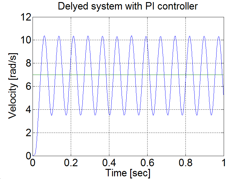
Conclusion AU = 1.7 and TU≈0.08. According to the table PPI=0.85 and IPI=12. Measurement results are shown in Figure 6-7.
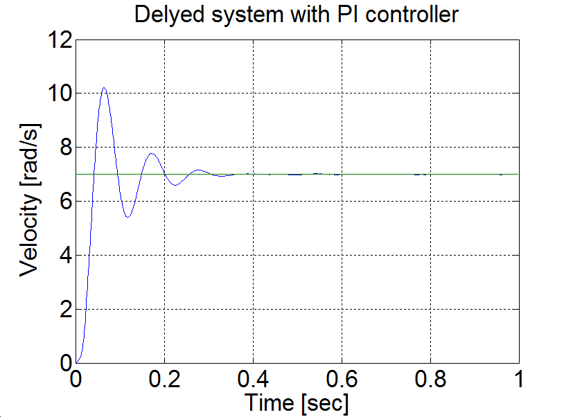
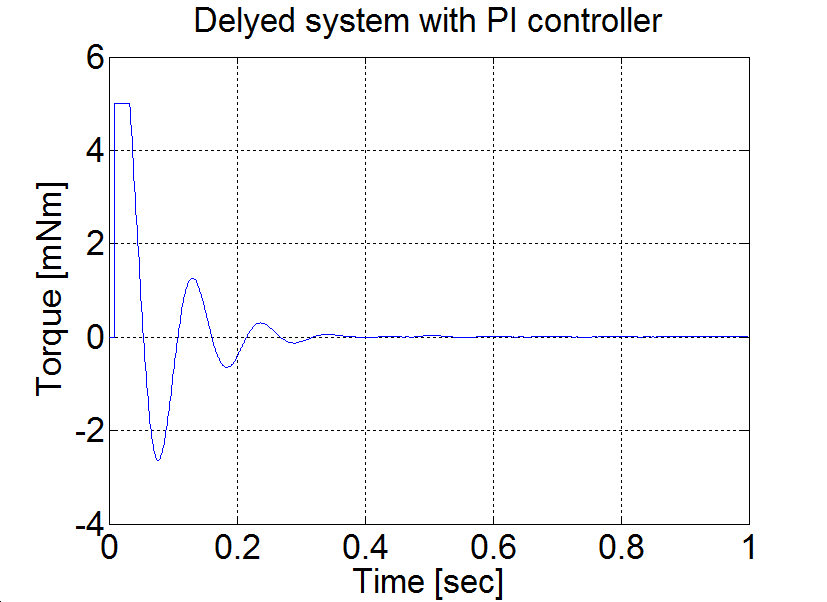
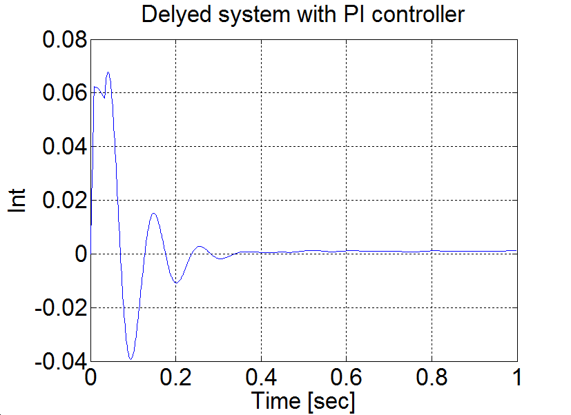
P control results
6.5.13. Sliding mode control results
Sliding mode control can be also applied. There are two different measurements. The control part of the measurements is the same, but since the velocity of the motor is calculated from position data, this makes the velocity diagram noisy. By applying a filter for the velocity the results are smoother.
Enter measurement length in milliseconds: 12000
The state variable names:
time (given)
position (given)
velocity (given)
torque (given)
sigma (selected)
The controller code is the following:
Declaration:
float sigma;
float error;
float error_dot;
float ref=5.0;
float lambda=2;
static double ini_0 = 0;
static double ini_1 = -10;
Controller:
if (ini_1 < 0)
{
ini_0 = ResultData.Position;
}
ini_1 = 5;
error=ref-ResultData.Position+ ini_0;
error_dot=- ResultData.Velocity;
sigma= error+ lambda*error_dot;
ResultData.StateVariable_5 = sigma;
if (sigma>0)
{ ResultData.Torque=0.1;
}
if (sigma<0)
{ ResultData.Torque =-0.1;
}
if (sigma=0)
{ ResultData.Torque=0;
}
Select item to download: All files
Please, download them by clicking the button “DOWNLOAD”
The results are plotted by the following MATLAB file:
% please, modify it according to you file names
sv_1_n0ktqaui51tw5hrtvpypxu45
sv_2_n0ktqaui51tw5hrtvpypxu45
sv_3_n0ktqaui51tw5hrtvpypxu45
sv_4_n0ktqaui51tw5hrtvpypxu45
sv_5_n0ktqaui51tw5hrtvpypxu45
time=time/1000;
plot(time,position)
set(gca, 'fontsize', [25]);
xlabel('Time [sec]');
ylabel('Position [rad]');
title('Sliding mode controller');
% you can adjust your axis
axis([0 12 0 6]);
grid
pause;
print -djpeg smc_poz
plot(time,velocity)
set(gca, 'fontsize', [25]);
xlabel('Time [sec]');
ylabel('Velocity [rad/s]');
title('Sliding mode controller');
% you can adjust your axis
axis([0 12 0 3]);
grid
print -djpeg smc_vel
pause;
plot(5-position,-velocity)
set(gca, 'fontsize', [25]);
xlabel('Position error [rad]');
ylabel('Velocity error [rad/s]');
title('Sliding mode controller');
% you can adjust your axis
axis([0 5 -3 0]);
grid
print -djpeg smc_traj
pause;
plot(time,torque)
set(gca, 'fontsize', [25]);
xlabel('Time [sec]');
ylabel('Torque [mNm]');
title('Sliding mode controller');
% you can adjust your axis
axis([0 12 -0.15 0.15]);
grid
print -djpeg smc_torque
pause;
plot(time,sigma)
set(gca, 'fontsize', [25]);
xlabel('Time [sec]');
ylabel('Sigma');
title('Sliding mode controller');
% you can adjust your axis
axis([0 12 -2.5 2.5]);
grid
print -djpeg smc_sigm
|
|
|
|
|
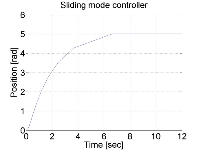
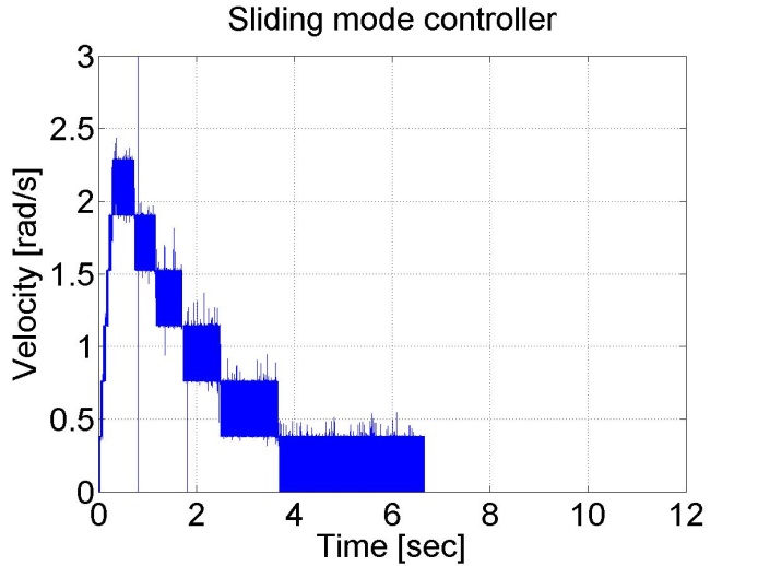
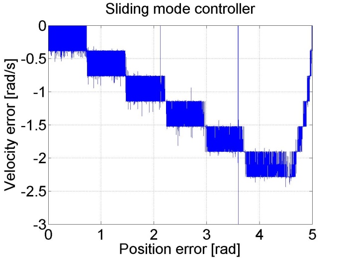
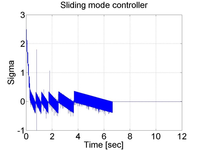
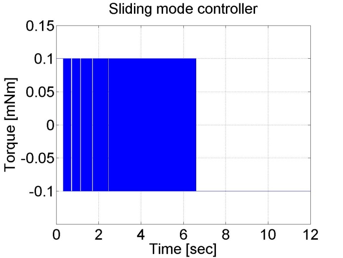
Figure 6-16. Results of the position controller with sliding mode controller
The sliding mode controller with the velocity filter has the following form:
Declaration:
float sigma;
float error;
float error_dot;
float ref=5.0;
float lambda=2;
/* filter variables*/
static float z_1=0.0, z_2=0.0, z_3=0.0;
static float ztmp_1=0.0, ztmp_2=0.0;
/*omega_c=10 unmodelled dynamics of the filter causes big chattering */
float Azd11= 1, Azd12= 0.0010, Azd13= 0.0000;
float Azd21= -0.0005, Azd22= 0.9999, Azd23= 0.0010;
float Azd31= -0.9851, Azd32= -0.2960, Azd33= 0.9703;
float Bzd1= 0.0000, Bzd2= 0.0005, Bzd3= 0.9851;
/* omega_c= 1/0.007 unmodelled dynamics of the filter does not cause big chattering
float Azd11= 0.9996, Azd12= 9.9072e-004, Azd13= 4.3344e-007;
float Azd21= -1.2637, Azd22= 0.9730, Azd23= 8.0496e-004;
float Azd31= -2.3468e+003, Azd32= -50.5468, Azd33= 0.6280;
float Bzd1= 4.3671e-004, Bzd2= 1.2637, Bzd3= 2.3468e+003;
*/
static double ini_0 = 0;
static double ini_1 = -10;
Controller:
if (ini_1 < 0)
{
ini_0 = ResultData.Position;
}
ini_1 = 5;
error=ref-ResultData.Position+ ini_0;
/* filter */
ztmp_1 = Azd11* z_1 +Azd12* z_2 +Azd13* z_3 + Bzd1*ResultData.Velocity ;
ztmp_2 = Azd21* z_1 +Azd22* z_2 +Azd23* z_3 + Bzd2*ResultData.Velocity ;
z_3 = Azd31*z_1 +Azd32*z_2 +Azd33* z_3 + Bzd3*ResultData.Velocity ;
z_1 = ztmp_1;
z_2 = ztmp_2;
ResultData.Velocity =z_1;
error_dot=- z_1;
sigma=error+ lambda*error_dot;
ResultData.StateVariable_5 = sigma;
if (sigma>0)
{ ResultData.Torque=0.1;}
if (sigma<0)
{ ResultData.Torque =-0.1;
}
if (sigma=0)
{ ResultData.Torque=0;}
The results can be seen in the figure below:
|
|
|
|
|

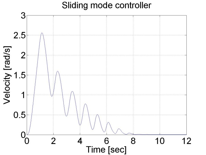
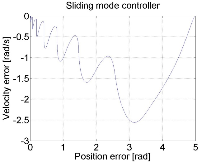
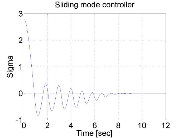
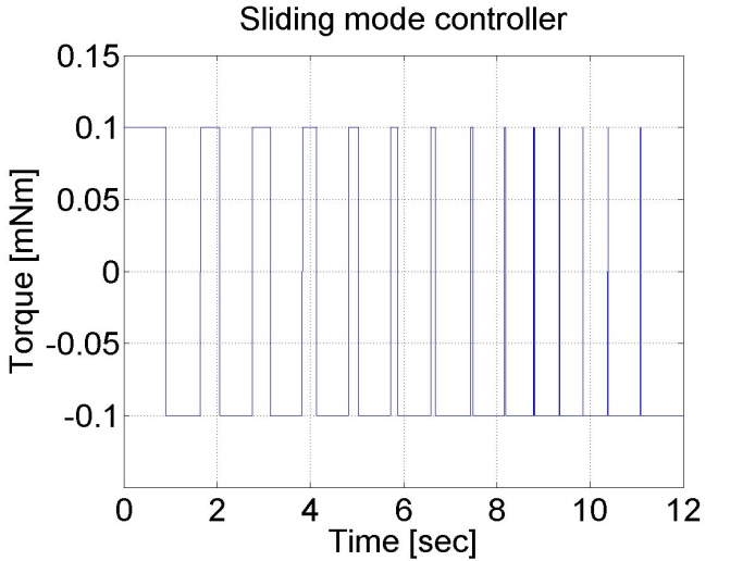
Figure 6-16. Sliding mode control with a velocity filter
|
|
|
|
|
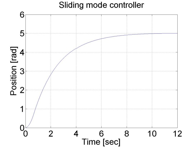
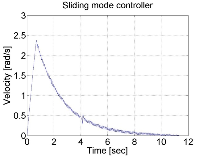
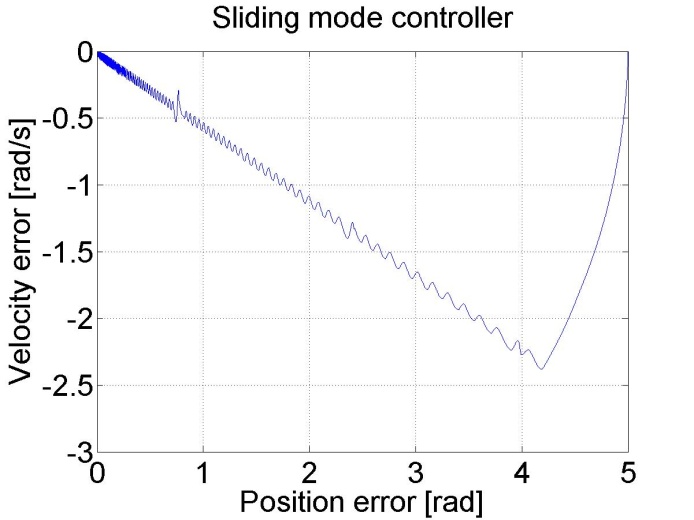
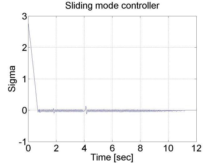
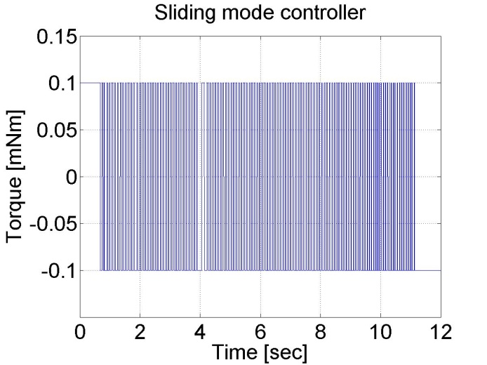
Figure 6-17. Results of the position controller with sliding mode controller with velocity filter
6.6. Complex design and measurement
In this section the theoretical basics of the DC motor control will be reviewed by focusing on the state feedback control. As the control of the motor is solved by a computer, the model expressed in discretized form. Furthermore the introduced methods will be implemented into MATLAB. In the theoretical review, only the necessary steps for implementation is emphasized. The more detailed description of methods can be found in the recommended literature.
6.6.1. State feedback and its design
Let us consider the following explicit Discrete time invariant state space model:
| (6.1) |
Where

: the state vector at k

: the column vector of the input signal at k

: the vector of the output signal at k,

: the system matrix,

: the input matrix,

: the output matrix,

: feedthrough matrix (usually 0),
The purpose of state feedback is to change the system matrix in a way that the behaviour of the system is favourable to us. Since the eigenvalues of  are the system’s poles, it is evident, that by changing the eigenvalues we can manipulate the behaviour of the system freely (with particular limits). From the state space equations it can be seen that if we choose
  to:
to:
| (6.2) |
then the value of  can be changed.
Thus we get:
| (6.3) |

Where:

: the feedback matrix

: the new input signal of the system,
The new system matrix is  , which value can be set with
  . Since K does not affect the system matrix directly - but after the multiplication with
  – it is not possible to have an arbitrary result.
Hence the condition for design and correct operation of a state feedback is the controllability of the system represented by the state space model. This means that the system can reach any state – with the proper input signal – from any given state in a finite interval. In case of a Discrete time system the condition of total state controllability is that the rank of controllability matrix  of the system is equal to the number of state variables (n):
| (6.4) |

Designing the state feedback is based on constructing the characteristic equation of our own ( ), where we choose the new placement of the poles. (The number of poles must remain the same of course.). This formula is usually based on the selection of two dominant poles; using these we define the behaviour of the system. Then we choose other auxiliary poles which have higher values than the dominant poles. (The necessity of the auxiliary poles are to keep the number of poles the same.)
Assigning values to the poles happen continuously in case of discrete controllers too, because the controlled plant is usually continuous in time. If we want a stable system, all of the poles must have a negative integer part. We can set the dominant pair of poles with the damping and time constant as well. Let us consider the following oscillating double storage:
| (6.5) |
If  , then the poles of the transfer function:
| (6.6) |
Where:
| (6.7) |
| (6.8) |

From the envelope of the unit jump’s response the  percentage time constant can be derived:
| (6.9) |

So if the values of  and
and  are given, then:
| (6.10) |

From this we can calculate the dominant pair of poles. We choose the further poles much larger, so the effect of these are not significant. If we have the poles in continuous time ( ), the same can be calculated in Discrete time (
 ) with the following formula:
| (6.11) |

where  is the sampling period.
The following task is to determine the value of  in a way that this can be achieved. In case of Single Input, Single Output (SISO) systems this may be easily reached: All we have to do is compare the
  system matrix’s poles (parameterized with
  ) with the chosen poles and calculate
  . This method is called the Ackermann formula:
| (6.12) |
Where  indicates the original system matrix substituted into the desired characteristic equation. In case of Multiple Input, Multiple Output (MIMO) systems determining
  is a more complex problem and in general only approximate solutions can be achieved; which means the actual values of the poles might be different from the desired ones.
6.6.2. Application of reference signal correction
With the previous procedure we get a system which poles’ are the ones we set. In case of controller design, it is expected that output signal of the whole system in the steady state match the reference signal. For this reason we need the so called reference signal correction. The state feedback controller with reference signal correction has the following structure:
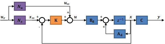


Where  is the value of the state vector and
  is the actuating signal value in steady-state. The feed-forward containing
  is crucial, because without it, the actuating signal is not in steady-state. (Basically it replaces an integrator.) The
  component calculates the goal values of the state variables according to the goal values of the output; hence it ensures that the input of
  is the error signal. It is worthy to note, that in case we use feed-forward alone (without the feedback) the system would eventually reach the end position as well; however not the way we planned.
So the goal is:
| (6.13) |

For this:
| (6.14) |


Determination of  :
:
| (6.15) |

Calculation of  :
:
| (6.16) |
Summarizing:
| (6.17) |
Where  is a n x m nullmatrix and
  is a m x m identity matrix.
6.6.3. Design of the state observer
In real life situations we usually do not have the opportunity to measure all the state variables. It has several reasons; e.g. technically it is not possible to measure the given state variable or it cannot be measured accurately enough, the measurement is not cost efficient or the physical meaning of the state variable is unknown (e.g. in case of artificially created, identification based state space models). In such cases we need a state observer; the general function of the state observer is to determine the state of the system using the input and output signals, which can be easily measured in most cases. Therefore the state observer has two inputs: the block input ( ) and output (
 ); the output of the state observer is the vector of the observed state variables (
 ).
).
A state observer can only be applied, if the system is observable. Formally, a system is said to be observable if, knowing the inputs and outputs of the system in finite time, the system’s initial state can be determined. In case of time invariant systems in Discrete time it is true when the rank of the system’s observability matrix is maximal, that is its rank is n:
| (6.18) |
The state observer in Discrete time :
| (6.19) |
The estimation error:
| (6.20) |
The goal is to keep the estimation error converging to zero ( ). Let us substitute the estimation error into the state observer equation and express it:
| (6.21) |

Since:
| (6.22) |

Therefore:
| (6.23) |

It follows that:
| (6.24) |

The last two term is always zero, if:
| (6.25) |
Furthermore our goal is to get  as fast as possible. This is valid when the system is stable and fast:
| (6.26) |
It can be ensured by proper selection of  . To have this we substitute
  and
and  in the equation of the estimation error:
| (6.27) |
We transpose the equation:
| (6.28) |
Let us compare this with the state feedback equation:
| (6.29) |
It is visible, that the two equations are very similar and we can use that to determine the value of  , using the methods applied in case of state feedback. Consider the following system:
| (6.30) |


If we design a state feedback for this system, the value of  is:
is:
| (6.31) |

The only important remaining issue is the pole placement. To decide this matter we should use the greatest absolute valued pole in continuous time (obtained in the primary state feedback design) and choose many orders of magnitude larger. Selecting it carefully plays a crucial role in the stability of the system, especially if the actual system is different from the model, because the slow observer causes an unstable system. Therefore it is a basic requirement for a state observer that it must operate faster than the observed system. With this we get the following controller:
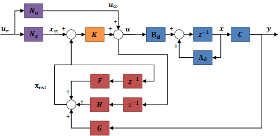


6.6.4. Integral control
Up to this point the designed controller works great theoretically: we decide the pole placement of the system, we determine how and how fast the system should reach steady state; and there is no steady-state error. What if the block is different from the one we used during design? In this case the state feedback will not place the poles to their designed location, since they are not in the place where we expect them to be; this may even lead to an unstable system and certainly lead to steady-state error, because the reference signal correction is based on the state space equations. On top of that, the state observer would not observe the real states.
The solution for the steady-state error is placing an integrator into the system. Using this we can eliminate the  part of the reference signal correction, since the integrator also has an output in case there is no error. In order to build in the integrator, introducing a new state variable is necessary:
| (6.32) |

Here the Discrete time integrator is based on the left hand endpoint method. Extending the block state space equations with this:
| (6.33) |
The state feedback have the following form:
| (6.34) |
Thus in this case we design the state feedback to this extended system and we use the obtained  and
and  matrices as follows:
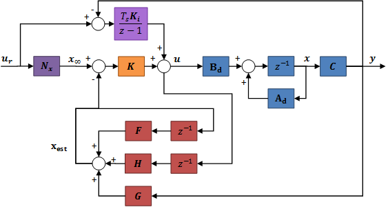


As we can see, the feed-forward containing  is replaced with the integrator, since the integrator ensures the lack of steady-state error. Placing the integrator in the feed-forward does not affect the design of the reference signal correction and the state observer.
6.6.5. Identification of the system
First we need to determine the model of the controller before the designing process can begin. To do that, we use the MATLAB System Identification Toolbox. The toolbox gives the possibility to identify systems from measurement results, which can be used for controller design. An important condition for this is to have a measurement which represents the system properly; since the program creates the system using the input and output values, any special phenomenon that does not occur in the measurement (but in the real system) is likely to not occur in the model as well. Before we start the measurement, it is practical to select the model we would use. In this case designing the controller would require a state space model in Discrete time . This can be easily derived from a transfer function. MATLAB offers several options to do that, we are going to use the ARMAX model. ARMAX is an acronym; it stands for AutoRegressive Moving-Average model with eXogenous inputs. A question regarding the emphasis of exogenous input may occur; hence before presenting the ARMAX model, we should understand two of its components, the AR and MA models. The AutoRegressive (AR) model:
| (6.35) |
Where:

is the output value at
 time step
is the internal input, white noise value at
 time step
As we can see, this is a stochastic process. The Moving-Average (MA) has the same structure:
| (6.36) |
Where . Since these models have no exogenous inputs, they are not suitable for describing the engine; however putting the models together and extending it with exogenous inputs we obtain the so called ARMAX model, which is eligible. The formula of the ARMAX model:
| (6.37) |

Where:

is the exogenous input

is the system delay
, here the first coefficient is not 1. The reason for this is to have an arbitrary amplification of the system.
The purpose of the  term containing the white noise input is to map the measurement error. Actually this is the error of the equation:
| (6.38) |
If there is no measurement error, then  :
:
| (6.39) |
Therefore the transfer function:
| (6.40) |
MATLAB can construct the transfer function for us, however understanding the basic operational principles may be useful. Substituting the values as parameters into the ARMAX equation, the magnitude of the error is given as a function of the polynomials coefficient. The value of the polynomials and thus the transfer function can be determined by minimizing the square of the error. The MATLAB does not determine the value of the delay time; it has to be given by the user.
From the transfer function we can develop a state space model in more than one way, e.g. observable canonical form, controllable canonical form, etc. In this methods, the physical meaning of the state variables are unknown; however this is not a disadvantage, since we do not expect this behaviour because of identification. In most cases the state space representation can be derived from the transfer function as follows:
| (6.41) |
Let:
| (6.42) |
With this:
| (6.43) |


Consider the state variables as follows:
| (6.44) |


Hence:
| (6.45) |


The state space model:
| (6.46) |
In possession of the state space model, the controller design may be performed.
6.6.6. Design of the control
After the review of the theoretical basics the design of the control can be done in the following three steps:
Identification of the system
Design and simulation of the control
Implementation and analysis of the control
These will be introduced in this section.
6.6.7. Identification of the motor
6.6.7.1. Analysis of the characteristics
First the system had to be analysed. The DC motor available via the internet. With the help of the working system, the control of the input signals can be written in C programming language. By sending the C code to the remote monitoring station, it will be compiled and the result will be sent back. In this case the input of the motor is the required moment. From this moment, the current controller computes the output voltage. Thus the damaging input signals are prohibited. While the controlled output is the velocity of the motor. The maximal achievable angular velocity in the case of constant input signal (100 mNm):
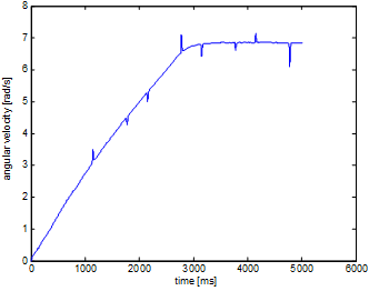
It can be noticed that the velocity is computed from the position by numerical differentiation and filtering. Therefore some pike still remain in the result. The designing of the filter will be detailed in later section.
In the case of 3 mNm :
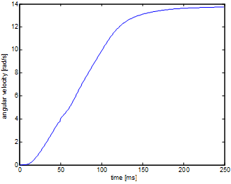
After more measurement, it can be stated that the maximum of the angular valocity is 14 rad/s. Furthermore it can be seen that the system gives higher response in the case of less moment. This means that the current control works wrong in the case of high input moments.
In the case of inversed direction of rotation (-3 mNm):
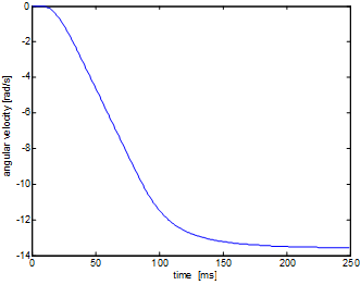
It can be seen that the absolute value of the extremes are about the same as in the previous case. In the next step, the system will be analysed by a quasi-static measurement to obtain the relation between the input moment and the output velocity. The measurement begin with a -3 mNm as an input and it increased slowly until +3 mNm:
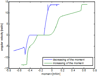
The figure above shows that the characteristic of the system is far away from linear:
Deadband: because of static friction.
There are more breakpoint.
Hysteresis: The direction of the moment change is also an important factor.
6.6.7.2. Design of the excitation for the identification
To achieve a well working control, the system has to be as linear as possible. Even the case of non linear system, every system can be linearized around a given working point. Thus, to demonstrate the operating of the control, a precision velocity controller will be made. At first the system is taken into the close area of the working point then the system pass to the precision control.
After the system is taken into the close area of the working point, a square wave signal is applied as input. The response of the system will be the basics of the identification. Then the picked linear section should be the linear section between 0.2mNm and 0.5mNm. For the identification of this, a square wave signal is used by setting of 4s as the time of period, 0.35mNm as the mid-torque and 0.15 as the amplitude. And 2 seconds was given to reach the working point:
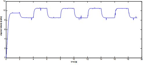
The 6-15.figure shows the output of the system. And this output well approximates the output of a linear system. The C code of the measurement is:
typedef struct
{
float Position;
float Velocity;
float Torque;
float StateVariable_5;
float StateVariable_6;
float StateVariable_7;
float StateVariable_8;
float StateVariable_9;
float StateVariable_10;
NewControllerData
NewControllerData CalculateController(
const float CurrentPosition,
const float OldPosition,
const float OldVelocity,
const float CurrentTime,
const float OldTime,
const float Old_StateVariable_5,
const float Old_StateVariable_6,
const float Old_StateVariable_7,
const float Old_StateVariable_8,
const float Old_StateVariable_9,
const float Old_StateVariable_10
NewControllerData ResultData; // result
//Filter coefficient
static float filB0 = 0, filB1 = 0.00013337, filB2 = 0.0012028, filB3 = 0.0009847099, filB4 = 7.3193E-05;
static float filA0 = 1, filA1 = -3.1152, filA2 = 3.6392, filA3 = -1.8895, filA4 = 0.36788;
//input
static float input0 = 0, input1 = 0, input2 = 0, input3 = 0, input4 = 0;
//filtered value
static float filter0 = 0, filter1 = 0, filter2 = 0, filter3 = 0, filter4 = 0;
float u;
//mid-value of the moment
float bias = 0.35;
//waiting for the set up
int start = 2000;
//time of the period
int period = 4000;
//amplitude
float amplitude = 0.15;
// Position is saved automatically
ResultData.Position = CurrentPosition;
// angular velocity is saved automatically
if (CurrentTime != 0.0f){
ResultData.Velocity = (1000.0f * (float)(CurrentPosition - OldPosition)/(float)(CurrentTime - OldTime));
}
else {
ResultData.Velocity = 0.0f;
}
//velocity filtering
input0 = ResultData.Velocity;
filter0 = (filB0 * input0 + filB1 * input1 + filB2 * input2 + filB3 * input3 + filB4 * input4 - (filA1 * filter1 + filA2 * filter2 + filA3 * filter3 + filA4 * filter4)) / filA0;
input4 = input3; input3 = input2; input2 = input1; input1 = input0;
filter4 = filter3; filter3 = filter2; filter2 = filter1; filter1 = filter0;
ResultData.StateVariable_5 = filter0;
//the moment
if(CurrentTime < start)
{
u = 0;
}
else
{
u = (((int)CurrentTime - start) % period - period / 2 > 0 ? amplitude : -amplitude);
}
ResultData.Torque = u + bias;
ResultData.StateVariable_6 = u;
return ResultData;
}6.6.7.3. Identification with the help of the MATLAB
First the results of the measurement have to be uploaded into the MATLAB. Then the transient phase should be cut off, it’s won’t be needed. Instead of the true velocity and moment, the their deviations from the working point is used for the identification of the system. Furthermore the sampling time is 1ms. By performing the previous steps, the iddata command can generate the neccessary data structure for the System Identification Toolbox. Thereafter the degrees of the polynomials should be specified for the ARMAX model ( is the degree of the
  ,
,  is the degree of the
  ,
,  is the degree of the
  ,
,  is the deadband). Then
  row vector can be composed, where
  and
and  . The higher values of the degree of the polynomial results in higher uncertainty of the identification, in which case the MATLAB shows the „Warning: Pole locations are more than 10% in error.” message. This is important because the pole locations has to be changed, and the method doesn’t work well if the poles aren’t in the right position. Fortunately the identification takes only a few seconds, so many types of the setting should be tried. The identification can be run with the help of armax command. The result of this command will be the data structure of the system, whereof the th2poly function compute the descriptive row vectors of the polinoms. In these, the coefficients are ordered according to descending exponent values of the
  terms, so the
  is the last term. Of course, there should be zero coefficients as well. Actually in the this step the numerator and the denominator of the discrete transfer function are obtained, thus the tf can compute the discreteized form of the transfer function. The MATLAB code of the identification is:
start=1800;                                 %point of begin
y=velocity2(start:end)-velocity2(start);    %measurement vector of the angular velocity
u=torque2(start:end)-torque2(start);        %vector of the moment
n=3;                                        %number of the states
Ts=0.001;                                   %sampling time
z=iddata(y,u,Ts);                           %upload of the measured data
nn=[n,1,1,1];                               %set the degrees of the polynoms
tharmax=armax(z,nn);                        %identification
[A,B,C]=th2poly(tharmax);                   %read of the polys
sys=tf(B,A,Ts);                             %transfer function
The transfer function is:
| (6.47) |
It is hard to see that this result is good or not. Therefore the response of the identified system should be computed by applying the input of the real system:
yid=idsim(tharmax,u,zeros(n,1)); %response of the identified system
t=0:Ts:(size(y)-1)*Ts; %time vector
figure(1); %new figure
plot(t,y,t,yid); %plot
legend('mesured','identified'); %legend
xlabel('time [s]'); %horizontal
ylabel('angular velocity [rad/s]'); %vertical
The operation of the identified system can be checked with the help of idsim function which calculate the output vector with respect of the input vector and initial states. Then the plot of the results is:
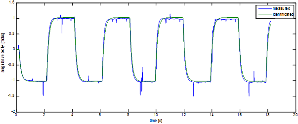
It can be seen in the figure that the model well approximate the experience. It has to be mentioned that the used excitation for the identification is can be optional, but it has to be suitable to specify the system features. So the result of the identification algorithm describe the real system well and with high degree of certainty in the case of the given exciting.
To design the control, it is necessary to know the discretized form of the state space model of the system, what can be obtained with the help of ss command:
sysd=ss(sys);                               %state space model
[Phi Gamma C D]=ssdata(sysd);               %read the matrices
Now everything ready for the design of the control.
6.6.8. Design of the control
6.6.8.1. Control without of the integrator
First the parameter of the required system has to be defined, then the pole of the continous time system also has to be defined. The response of the reqiured system is:
a=2;                                        %percentage of the set up
Tap=0.2;                                    %time of control
xi=0.8;                                     %dumping
w0=log(100/a)/Tap/xi;                       %natural frequency

sdom1=-w0*xi+1i*w0*sqrt(1-xi^2);            %dominant pole
sdom2=conj(sdom1);
scinf=-4*w0;                                %auxiliary pole to control
soinf=scinf*5;                              %auxiliary pole to observe
if(-soinf>0.5/Ts)                           %Shannon-theory check
    display('Sampling time is too short!');
end;

%model of the required system
tcsys=zpk([],[sdom1, sdom2, scinf*ones(1,n-2)],-w0^2*scinf^(n-2));
figure(2);                                  %new plot
step(tcsys);                                %step response
The response of the step function is:
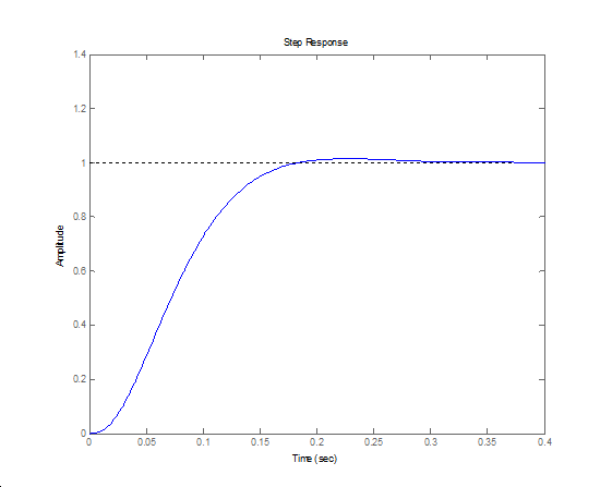
Then the poles in discretized time is:
%calculation of the poles for discrete time
zdom1=exp(sdom1*Ts);
zdom2=exp(sdom2*Ts);
zcinf=exp(scinf*Ts);
zoinf=exp(soinf*Ts);
Then the state feedback, the reference signal correction and state observation are can be done according to the theoretical introduction:
%checking of controllability
Mc=ctrb(Phi,Gamma);
if rank(Mc)~=n
disp('The system can not be controlled!');
end
%design of the state feedback
phic=[zdom1 zdom2 zcinf*ones(1,n-2)]; %new poles
K=acker(Phi,Gamma,phic); %pole placement
%calculation of the base-signal correction
NxNu=inv([Phi-eye(n) Gamma;C 0])*[zeros(n,1);1];
Nx=NxNu(1:n);
Nu=NxNu(n+1);
%checking of observability
Mo=obsv(Phi,C);
if rank(Mo)~=n
disp('The system can not be observed!');
end
%design of state observer
phio=ones(1,n)*zoinf; %poles of the observer
G=acker(Phi',Phi'*C',phio)'; %pole transfer on dual system
F=Phi-G*C*Phi;
H=Gamma-G*C*Gamma;
At this point the design of the control is finished. To check the control, it is recommended to done some simulation in the Simulink.
Build the following model:
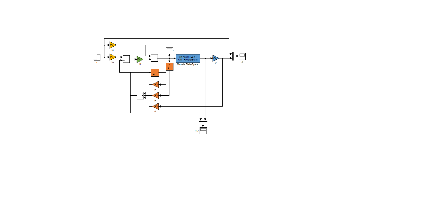
The section is divided to two parts. In the Discrete time state space model every states are taken out which useful to check the operation of the state estimator. While the signal which contains the C gain is the output. Take care of that the sampling time is given for every element! Thereafter the results are:
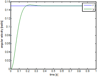
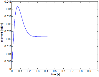
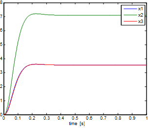
The control works well, the intervening signal doesn’t run over the linear section.
6.6.9. Integral control
For the design of the integral control, at first the equation of the state has to be expanded with the integrator:
iPhi=[Phi, zeros(n,1); Ts*C, 1];
iGamma=[Gamma; 0];
iC=[C 0];
To design the state feedback, one more pole is necessary:
siinf=scinf;                                %Pole for integrator
ziinf=exp(siinf*Ts);
if(-min([siinf soinf])>0.5/Ts)              %checking of Shannon-theory
    display('The sampling time is too short!');
end;
Then the state feedback control can be design:
iPhic=[zdom1 zdom2 zcinf*ones(1,n-2) ziinf];%new poles
iK=acker(iPhi,iGamma,iPhic);                %pole placement
K=iK(1:n);                                  %state feedback
Ki=iK(n+1);                                 %integrator feedback
The modified Simulink model is:
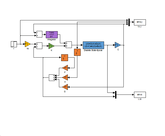
The results of the simulation are:
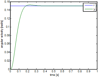
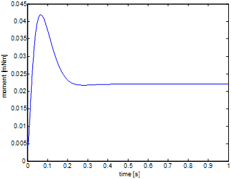
It can been seen that the response of the system doesn’t change. The difference will be noticeable if there were a 0.01mNm mistake in the calculation of the working point. In which case the response of the system without the integrator is:
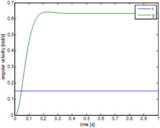
While the response of the system with the integrator is:
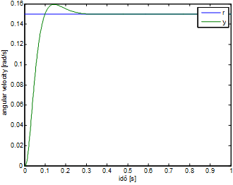
The figures above are clearly show that the response with the integrator is close to the ideal, while the control without the integrator is applicable only in the ideal case.
6.6.10. Filter design for velocity measurement
The angular velocity is computed from the position by numerical derivating. Therefore the input should be noisy. Thus this input has to be filtered. To design the filter, there are two controversial requirement: in the one hand the filter has to be as fast as possible because the delay caused by the filter reduce the stability of the system. On the other hand the noise has to be well filtered. The simplest filter can be achived by series connecting of the single capacity elements. Where -20dB/decade is the change of the amplification of the single capacity element. This type of the filter can be designed with the help of MATLAB. The continuous and discrete transfer functions can be calculated from value of the degree and locations of the poles:
filT=0.001;                                 %filter time constant
filN=3;                                     %filter degree

%continous time filter
filsys=tf(zpk([],-ones(1,filN)/filT,(1/filT)^filN));
dfilsys=c2d(filsys,Ts,'zoh');               %discrete time version
The implementation of the filter can be done after the discrete transfer function is obtained, but first analyse the operation of the filter (Bode diagram, step response and noisy input response):
figure(1);
dbode(dfilsys.num{1},dfilsys.den{1},Ts)     %Bode diagram

figure(2);
step(dfilsys);                              %step response

figure(3);
v=velocity(start:end)-velocity(start);      %noisy signal
lsim(dfilsys,v,t);                          %filtering of noisy signal
The results are:
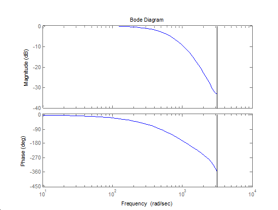
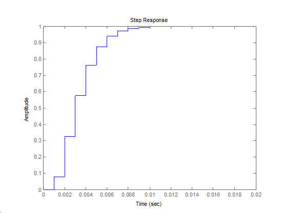
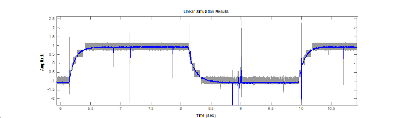
6.6.11. Implementation
The integration of the control can be written in C language. Although the online test environment has some limit. There aren’t possible to use arrays, it is impossible to define own functions or global variables. Therefore it is well recommended to create a program which translate the MATLAB code into C code. This program is introduced in the appendix.
6.6.12. Control without integrator
C code
#include <windows.h>
#include <stdio.h>
#include <rtapi.h>
#include <math.h>
#include <string.h>
#define PI 3.14159265358979323846
typedef struct
{
float Position;
float Velocity;
float Torque;
float StateVariable_5;
float StateVariable_6;
float StateVariable_7;
float StateVariable_8;
float StateVariable_9;
float StateVariable_10;
} NewControllerData;
NewControllerData CalculateController(
const float CurrentPosition,
const float OldPosition,
const float OldVelocity,
const float CurrentTime,
const float OldTime,
const float Old_StateVariable_5,
const float Old_StateVariable_6,
const float Old_StateVariable_7,
const float Old_StateVariable_8,
const float Old_StateVariable_9,
const float Old_StateVariable_10
)
{
NewControllerData ResultData; // result
static float filB0 = 0, filB1 = 0.080301, filB2 = 0.1544, filB3 = 0.017881;
static float filA0 = 1, filA1 = -1.1036, filA2 = 0.40601, filA3 = -0.049787;
static float input0 = 0, input1 = 0, input2 = 0, input3 = 0;
static float filter0 = 0, filter1 = 0, filter2 = 0, filter3 = 0;
static float Nu0_0 = 0.14662;
static float Nx0_0 = 23.677, Nx1_0 = 47.353, Nx2_0 = 23.677;
static float K0_0 = -1.2522, K0_1 = 0.81068, K0_2 = -0.37451;
static float F0_0 = 2.7896, F0_1 = -1.889, F0_2 = 0.84863, F1_0 = 2, F1_1 = -0.94991, F1_2 = 0, F2_0 = 0, F2_1 = 0.13587, F2_2 = 0;
static float G0_0 = 26.977, G1_0 = 44.981, G2_0 = 17.242;
static float H0_0 = 0.0625, H1_0 = 0, H2_0 = 0;
static float Gamma0_0 = 0.0625, Gamma1_0 = 0, Gamma2_0 = 0;
static float Phi0_0 = 2.7896, Phi0_1 = -1.3193, Phi0_2 = 0.84863, Phi1_0 = 2, Phi1_1 = 0, Phi1_2 = 0, Phi2_0 = 0, Phi2_1 = 0.5, Phi2_2 = 0;
static float C0_0 = 0, C0_1 = 0, C0_2 = 0.042236;
static float r = 0;
static float xu = 0;
static float xuL = 0;
static float xk0 = 0, xk1 = 0, xk2 = 0;
static float xkL0 = 0, xkL1 = 0, xkL2 = 0;
static float y = 0;
// Position is saved automatically
ResultData.Position = CurrentPosition;
// Angular velocity is saved automatically
if (CurrentTime != 0.0f){
ResultData.Velocity = (1000.0f * (float)(CurrentPosition - OldPosition)/(float)(CurrentTime - OldTime));
}
else {
ResultData.Velocity = 0.0f;
}

r=sin(CurrentTime/1000)/2-1;
input0 = ResultData.Velocity;
filter0 = (filB0 * input0 + filB1 * input1 + filB2 * input2 + filB3 * input3 - (filA1 * filter1 + filA2 * filter2 + filA3 * filter3)) / filA0;
input3 = input2; input2 = input1; input1 = input0;
filter3 = filter2; filter2 = filter1; filter1 = filter0;
if(CurrentTime < 2000) ResultData.Torque =   3.5000e-001;
else
{
y = filter0 +   -9.5218e+000;
xk0 = F0_0 * xkL0 + F0_1 * xkL1 + F0_2 * xkL2 + H0_0 * xuL + G0_0 * y;
xk1 = F1_0 * xkL0 + F1_1 * xkL1 + F1_2 * xkL2 + H1_0 * xuL + G1_0 * y;
xk2 = F2_0 * xkL0 + F2_1 * xkL1 + F2_2 * xkL2 + H2_0 * xuL + G2_0 * y;
xu = Nu0_0 * r + K0_0 * (Nx0_0 * r - xk0) + K0_1 * (Nx1_0 * r - xk1) + K0_2 * (Nx2_0 * r - xk2);
if(xu > 1) xu = 1;
if(xu < -1) xu = -1;
ResultData.Torque = xu +   3.5000e-001;
xuL = xu;
xkL0 = xk0;
xkL1 = xk1;
xkL2 = xk2;
}
ResultData.StateVariable_5 = r;
ResultData.StateVariable_6 = y;
return ResultData;
}
6.6.13. Results of the measurement

As the figure show the control well approximate the reference signal in spite of the facts there are no integrator in the control loop and modelled system is different from the real one. And of course the bigger deviation from the working point cause bigger error between the output and the reference signals.
6.6.14. Control with the integrator
C code
#include <windows.h>
#include <stdio.h>
#include <rtapi.h>
#include <math.h>
#include <string.h>
#define PI 3.14159265358979323846
typedef struct
{
float Position;
float Velocity;
float Torque;
float StateVariable_5;
float StateVariable_6;
float StateVariable_7;
float StateVariable_8;
float StateVariable_9;
float StateVariable_10;
} NewControllerData;
NewControllerData CalculateController(
const float CurrentPosition,
const float OldPosition,
const float OldVelocity,
const float CurrentTime,
const float OldTime,
const float Old_StateVariable_5,
const float Old_StateVariable_6,
const float Old_StateVariable_7,
const float Old_StateVariable_8,
const float Old_StateVariable_9,
const float Old_StateVariable_10
)
{
NewControllerData ResultData; // result
static float filB0 = 0, filB1 = 0.080301, filB2 = 0.1544, filB3 = 0.017881;
static float filA0 = 1, filA1 = -1.1036, filA2 = 0.40601, filA3 = -0.049787;
static float input0 = 0, input1 = 0, input2 = 0, input3 = 0;
static float filter0 = 0, filter1 = 0, filter2 = 0, filter3 = 0;
static float Nu0_0 = 0.14662;
static float Nx0_0 = 23.677, Nx1_0 = 47.353, Nx2_0 = 23.677;
static float K0_0 = 0.2386, K0_1 = -0.5816, K0_2 = 0.9255, K0_3 = 1.9278;
static float F0_0 = 2.7896, F0_1 = -1.889, F0_2 = 0.84863, F1_0 = 2, F1_1 = -0.94991, F1_2 = 0, F2_0 = 0, F2_1 = 0.13587, F2_2 = 0;
static float G0_0 = 26.977, G1_0 = 44.981, G2_0 = 17.242;
static float H0_0 = 0.0625, H1_0 = 0, H2_0 = 0;
static float Gamma0_0 = 0.0625, Gamma1_0 = 0, Gamma2_0 = 0;
static float Phi0_0 = 2.7896, Phi0_1 = -1.3193, Phi0_2 = 0.84863, Phi1_0 = 2, Phi1_1 = 0, Phi1_2 = 0, Phi2_0 = 0, Phi2_1 = 0.5, Phi2_2 = 0;
static float C0_0 = 0, C0_1 = 0, C0_2 = 0.042236;
static float r = 0;
static float xu = 0;
static float xuL = 0;
static float xk0 = 0, xk1 = 0, xk2 = 0;
static float xkL0 = 0, xkL1 = 0, xkL2 = 0;
static float y = 0;
static float i = 0;
// Position is saved automatically
ResultData.Position = CurrentPosition;
// Angular velocity is saved automatically
if (CurrentTime != 0.0f){
ResultData.Velocity = (1000.0f * (float)(CurrentPosition - OldPosition)/(float)(CurrentTime - OldTime));
}
else {
ResultData.Velocity = 0.0f;
}

r=sin(CurrentTime/1000)/2-1;
input0 = ResultData.Velocity;
filter0 = (filB0 * input0 + filB1 * input1 + filB2 * input2 + filB3 * input3 - (filA1 * filter1 + filA2 * filter2 + filA3 * filter3)) / filA0;
input3 = input2; input2 = input1; input1 = input0;
filter3 = filter2; filter2 = filter1; filter1 = filter0;
if(CurrentTime < 2000) ResultData.Torque =   3.5000e-001;
else {
y = filter0 +   -9.5218e+000;
xk0 = F0_0 * xkL0 + F0_1 * xkL1 + F0_2 * xkL2 + H0_0 * xuL + G0_0 * y;
xk1 = F1_0 * xkL0 + F1_1 * xkL1 + F1_2 * xkL2 + H1_0 * xuL + G1_0 * y;
xk2 = F2_0 * xkL0 + F2_1 * xkL1 + F2_2 * xkL2 + H2_0 * xuL + G2_0 * y;
i += 0.0019278 * (r - y);
xu = i + K0_0 * (Nx0_0 * r - xk0) + K0_1 * (Nx1_0 * r - xk1) + K0_2 * (Nx2_0 * r - xk2);
if(xu > 1) xu = 1;
if(xu < -1) xu = -1;
ResultData.Torque = xu +   3.5000e-001;
xuL = xu;
xkL0 = xk0;
xkL1 = xk1;
xkL2 = xk2;
}
ResultData.StateVariable_5 = r;
ResultData.StateVariable_6 = y;
return ResultData;
}
6.6.15. Results of the measurement in the case of integrator
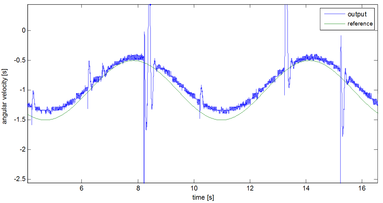
The control with the integrator works well and the error between the reference and output signal is neglactable.
6.6.16. Appendix
The complete MATLAB code of the control
%%settings
integrator=true;
idplots=true;
stateplots=true;
outplots=true;
filterdesign=true;
%% Identification
start=1800;                                 %start time
y=velocity2(start:end)-velocity2(start);    %vector of the measured angular velocity
u=torque2(start:end)-torque2(start);        %vector of the measured torque

n=3;                                        %number of state variables
Ts=0.001;                                   %sampling time
z=iddata(y,u,Ts);                           %measured data
nn=[n,1,1,1];                               %determination of degree numbers
tharmax=armax(z,nn);                        %identification
[A,B,C]=th2poly(tharmax);                   %polynomials read
sys=tf(B,A,Ts);                             %transfer function

yid=idsim(tharmax,u,zeros(n,1));            %response of the identified system
t=0:Ts:(size(y)-1)*Ts;                      %time vector
if(idplots)
figure(1);                                  %new diagram
plot(t,y,t,yid);                            %diagram
legend('measured','identified');            %legend
xlabel('time [s]');                         %x axis
ylabel('angular velocity [rad/s]'           %y axis
end;
sys

%%design of filter
if(filterdesign)
filT=0.001;                                 %filter time constant
filN=3;                                     %filter degree

%continous  time filter
filsys=tf(zpk([],-ones(1,filN)/filT,(1/filT)^filN));
dfilsys=c2d(filsys,Ts,'zoh');               %discrete time version

figure(1);
dbode(dfilsys.num{1},dfilsys.den{1},Ts)     %Bode diagram

figure(2);
step(dfilsys);                              %step response

figure(3);
v=velocity(start:end)-velocity(start);      %noisy signal
lsim(dfilsys,v,t);                          %filtering of the noisy signal
end;
%%design of controller
sysd=ss(sys);                               %model of state space
[Phi Gamma C D]=ssdata(sysd);               %read matrixes

a=2;                                        %what percent we stand
Tap=0.2;                                    %control time
xi=0.8;                                     %mitigation
w0=log(100/a)/Tap/xi;                       %own frequency

sdom1=-w0*xi+1i*w0*sqrt(1-xi^2);            %dominant poles
sdom2=conj(sdom1);
scinf=-4*w0;                                %auxiliary poles for the controller
soinf=scinf*5;                              %auxiliary poles for the observer
siinf=scinf;                                %auxiliary poles for the integrator
%checking of Shannon-theory
if(-soinf>0.5/Ts || (integrator && -min([siinf soinf])>0.5/Ts))
    display('The  settling time is too short!');
end;

%model of the target system with unit grain
if(idplots)
tcsys=zpk([],[sdom1, sdom2, scinf*ones(1,n-2)],-w0^2*scinf^(n-2));
figure(2);                                  %new diagram
step(tcsys);                                %calculation of the step response
end;

%calculating of the poles for discrete time
zdom1=exp(sdom1*Ts);
zdom2=exp(sdom2*Ts);
zcinf=exp(scinf*Ts);
zoinf=exp(soinf*Ts);
ziinf=exp(siinf*Ts);

%checking of controllability
Mc=ctrb(Phi,Gamma);
if rank(Mc)~=n
   disp(‘The system is uncontrollable!');
end

%design of the state feedback
if(integrator)
iPhi=[Phi, zeros(n,1); Ts*C, 1];
iGamma=[Gamma; 0];
iC=[C 0];
iPhic=[zdom1 zdom2 zcinf*ones(1,n-2) ziinf];%new poles
iK=acker(iPhi,iGamma,iPhic);                %pole placement
K=iK(1:n);                                  %state feedback
Ki=iK(n+1);                                 %feedback of the integrator
else
phic=[zdom1 zdom2 zcinf*ones(1,n-2)];       %new poles
K=acker(Phi,Gamma,phic);                    %pole placement
end

%calculating of the base-signal correction
NxNu=inv([Phi-eye(n) Gamma;C 0])*[zeros(n,1);1];
Nx=NxNu(1:n);
Nu=NxNu(n+1);

%checking of observability
Mo=obsv(Phi,C);
if rank(Mo)~=n
   disp(‘The system can not be observed!');
end

%design of state observer
phio=ones(1,n)*zoinf;                       %poles of the observer
G=acker(Phi',Phi'*C',phio)';                %pole transfer on dual system
F=Phi-G*C*Phi;
H=Gamma-G*C*Gamma;


%% simulation
if(integrator)
    open('szabint');
    sim('szabint');
else
    open('szab');
    sim('szab');
end;
rout=simruy(:,1);
uout=simruy(:,2);
yout=simruy(:,3);
tout=[0; tout];

if(outplots)
figure(3);
plot(tout,rout,tout,yout);
xlabel('time [s]');
ylabel('angular velocity [rad/s]');
legend('r','y');

figure(4);
plot(tout,uout);
xlabel('time [s]');
ylabel('torque [mNm]');
end;

if(stateplots)
figure(5);
plot(tout,simxo(:,1:n));
xlabel('time [s]');
ylabel('');
legend('x1','x2','x3');

figure(6);
plot(tout,simxo(:,n+1:2*n));
xlabel('time [s]');
ylabel('');
legend('x1','x2','x3');
end;
Chapter 7. Modelling Induction Motors
7.1. The AC Induction Motor
Asynchronous motors are based on induction. The least expensive and most widely spread induction motor is the so-called ‘squirrel cage’ motor. A typical asynchronous motor is shown in Figure 7-1. A metal ring at the ends resulting in a short circuit connects the wires along the rotor axis. There is no current supply needed from outside the rotor to create a magnetic field in the rotor. This is the reason why this motor is so robust and inexpensive. The stator phases create a magnetic field in the air gap rotating at the speed of the stator frequency (1).
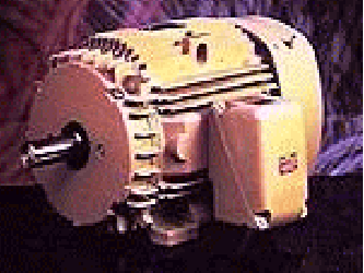
The changing field induces a current in the cage wires, which then results in the formation of a second magnetic field around the rotor wires. As a consequence of the forces created by these two fields, the rotor starts rotating in the direction of the stator field but at a slower speed (). If the rotor revolved at the same frequency as the stator, then the rotor field would be in phase with the stator field and no induction would be possible. The difference between the stator and the rotor frequency is called slip frequency (slip= 1-). There are several ways to control an induction motor in torque, speed or position, which can be categorized into two groups: there are scalar and vector control methods. Because of its outstanding robustness among all AC Motors, as can be seen in the Figure 7-2., the asynchronous ‘squirrel cage’ induction motor was chosen for detailed analysis and for control purposes. Further, the experimental application of this motor type has growing significance.
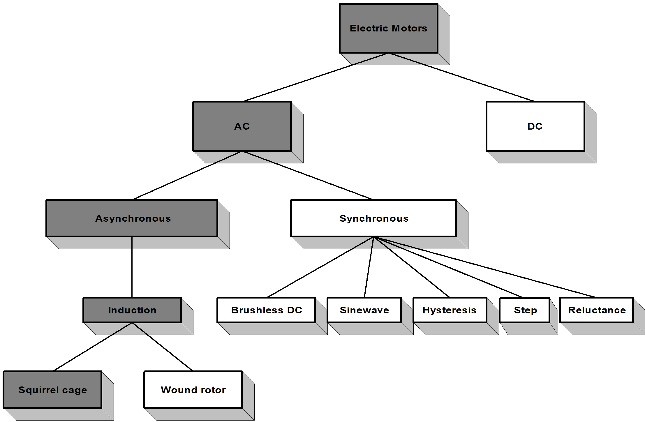
The following section will briefly describe this motor with the purpose of a deeper insight into its behavior later on.
7.2. General equations of AC Motors
The asynchronous or AC induction motor is represented by a stator and a concentric rotor with three-phase windings and a narrow airgap between the smooth surfaces of the rotor and the stator. Only the stator windings are fed by a voltage or current source inverter. The connection between the stator and the rotor is made by the flux, which means there is no mechanical connection between them apart from the bearings. For deducing the general equations of the AC induction motor (with “squirrel cage” rotor), let as make the following assumptions:
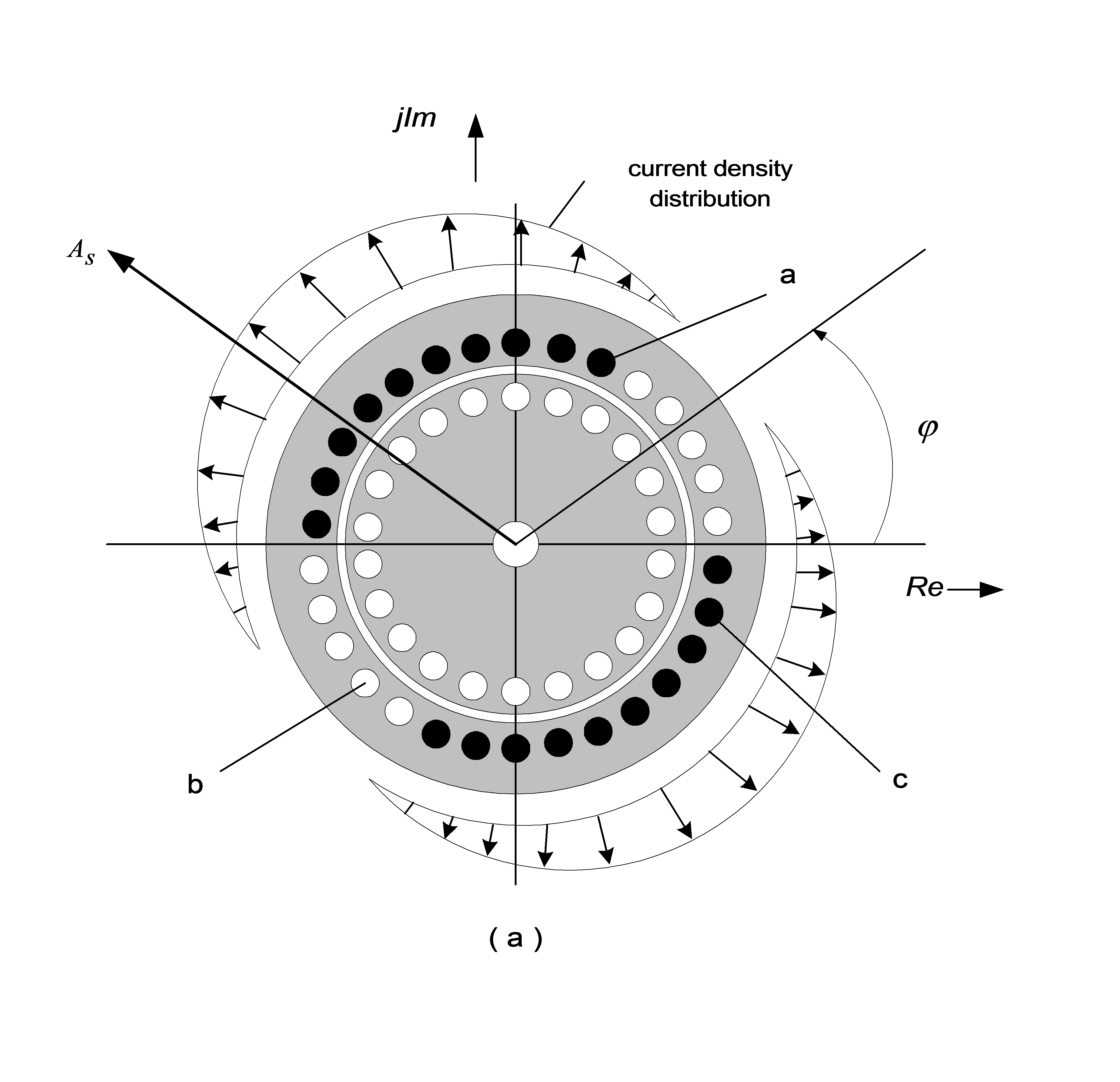
Presume a symmetrical three-phase windings system in the machine.
neglect the cooper losses and the slots in the machine;
spatial distribution of fluxes and amperturns wave are considered sinusoidal, as can be seen in Figure 7-3, the cross section of an Induction motor is shown in Figure 7-4.;
all the calculations based on the three-phased vector theory;
all the losses due to wiring, saturation, and slot effects can be neglected;
stator and rotor permeability are assumed to be infinite.
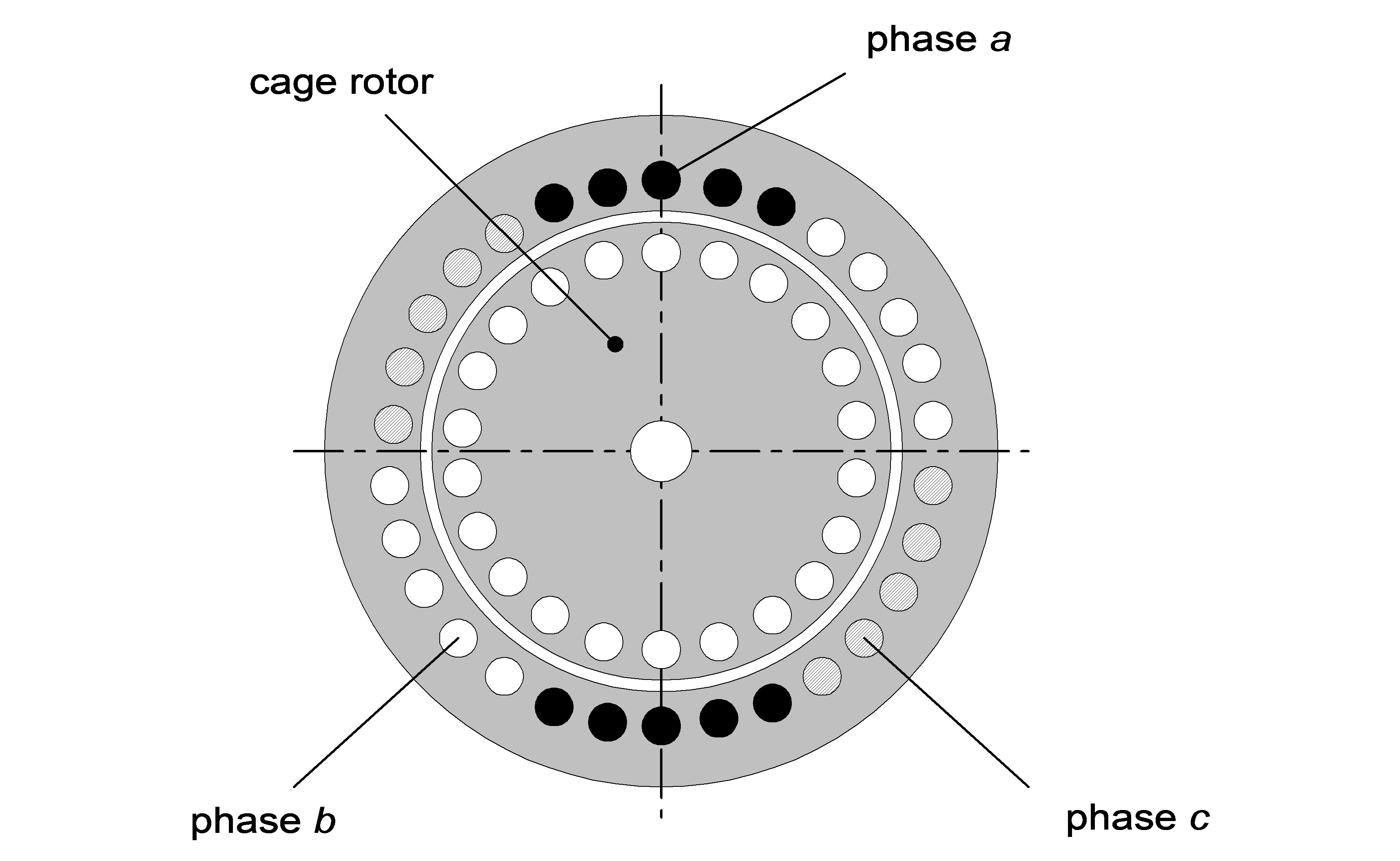
7.2.1. Machine equations in a natural co-ordinate system
The voltage equations of the stator are the following:
| (7.1) |
| (7.2) |

| (7.3) |
where  are the total fluxes of each phase including the main field of the windings and the leakage flux connection with the other windings, and
  is the one phase winding resistance. If we describe the above equations (7.1)(7.2)(7.3) according to the vector theory, the stator vectorial voltage equation will be the following:
| (7.4) |
| (7.5) |
where the latter equation is the zero sequence component.
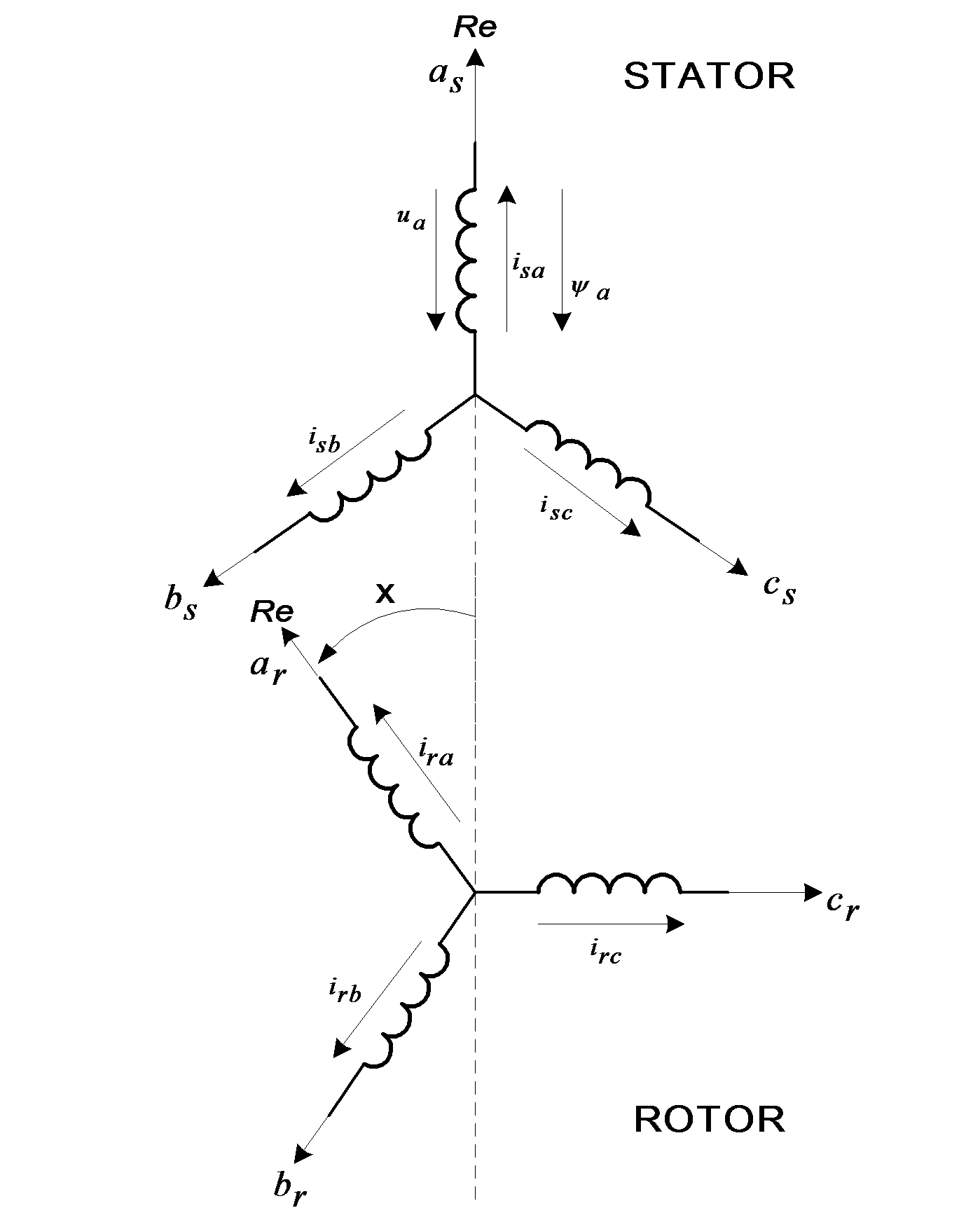
In practice, the zero sequence component can be neglected, so the equation (7.5) can be ignored and only one vectorial equation will describe the motor behavior instead of three phase equations. Writing the equation for rotor windings and proceeding like before we can easily obtain the vectorial voltage equation of the rotor:
| (7.6) |
| (7.7) |
where, for the same reason as before, the equation (7.7) can be ignored. The currents circulating in the three stator and three rotor windings generate the fluxes in the motor. We suppose that the air-gap is constant and the spatial distribution of the main magnetic field is sinusoidal, so the mutual inductance is proportional with the cosine value of the angle between two windings. Let us choose the real axes of the complex plane to match with the “a” phase axes. In the following discussion, we will call Natural Co-ordinate System the complex co-ordinate system fixed in this way to the “abc” axes of the motor. According to this agreement, the flux of phase “a” of the stator flux vector will be given by the equation (7.8), (7.9):
| (7.8) |
| (7.9) |
The motor’s general equations are defined by (7.4), (7.6), (7.8), (7.9). If  are given and the time function
 is also given, then the above equations unambiguously define the motor currents. They form a linear differential equation system with time dependent coefficients. If
  is not known or not given and must be calculated from the torque or motion equation, then the above equation system becomes nonlinear. The
  factor from the flux equations should be eliminated if the stator and rotor quantities are evaluated in the same co-ordinate system.
7.2.2. Machine Equations in a common co-ordinate system
In the previous section the stator quantities were given in their own complex co-ordinate system with the real axes fixed to the “a” phase axes of the stator windings. Let the  function describe the angular position of the new common co-ordinate system, referring to the fixed “a” phase axes. In this new common co-ordinate system the
  stator current vector angle, written as a complex number, became
  instead of the former
  . So this angle can be expressed as * = - xk.
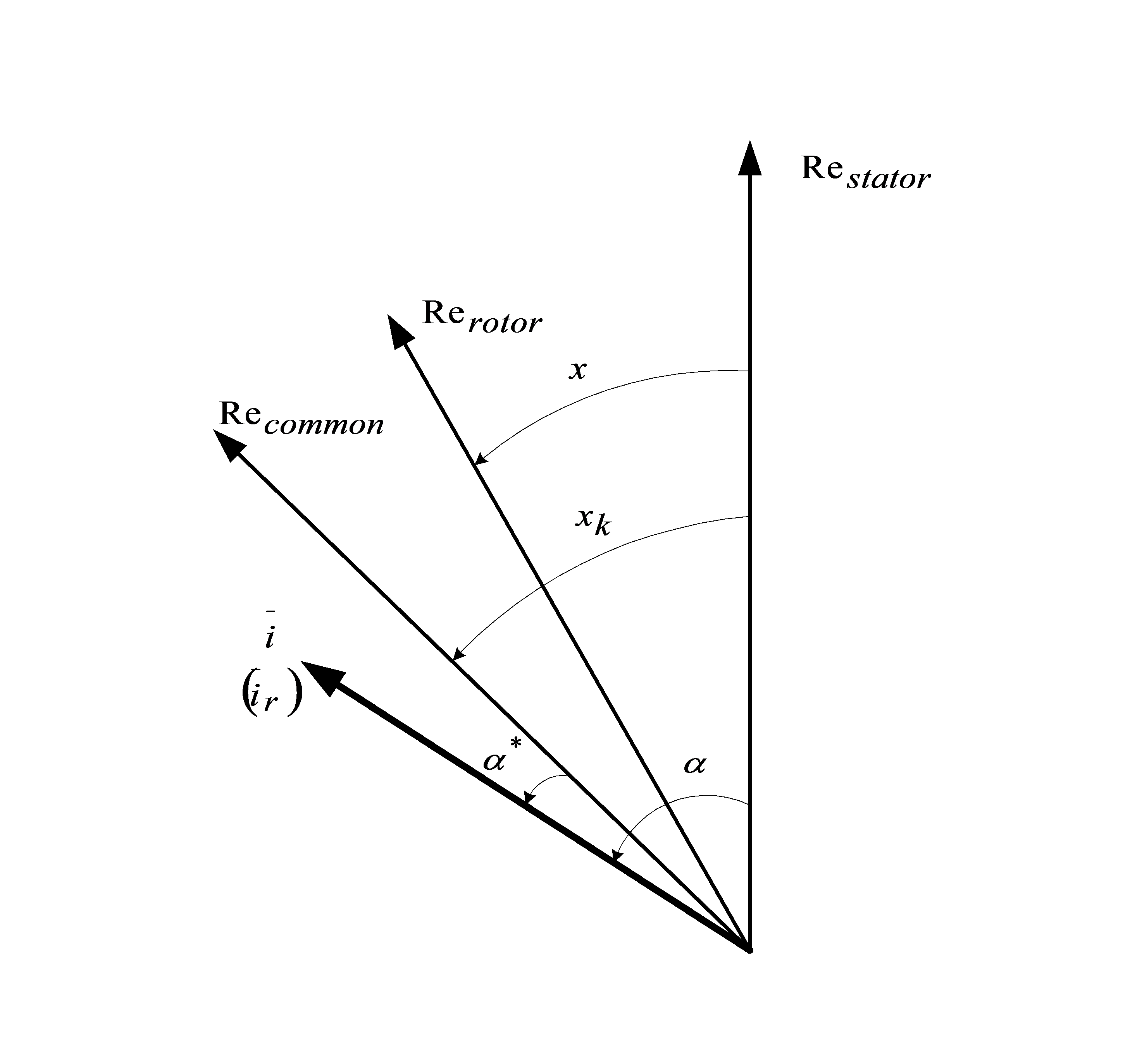
Now if we denote the current vector with  in the new reference frame, then the stator quantities can be expressed as
| (7.10) |

| (7.11) |

The angle between the two (fixed to the stator, common) co-ordinate systems is xk-x, so the rotor quantities can be expressed as
| (7.12) |

| (7.13) |

Having expressed the old quantities of the flux equation, in the new co-ordinate system, after a few simplifications, we obtain the following flux equations in the new common co-ordinate system:
| (7.14) |
| (7.15) |
If we look carefully at these equations, we can observe that the time dependent coefficients are not present in the equations anymore. So the flux equations of the asynchronous motor became as simple as in the case of a transformer. Let us have a look at the voltage equations, because they have become slightly complicated:
| (7.16) |
| (7.17) |
where dx/dt = is the rotor speed or angular velocity, and dxk/dt=k is the speed or angular velocity of the co-ordinate system. Both of these should be time dependent variables.
| (7.18) |
| (7.19) |
Looking at these equations we can see that the time dependent coefficients are present in the voltage equations, due to  . Supposing that the speed of the rotor in most cases is constant or cannot change dramatically, and choosing a co-ordinate system with a constant speed we obtain a constant coefficient linear differential equation system. Looking at the voltage equation, it can be observed that the flux has two components. The
  component is the transformation component, and the following
  component is the induced voltage, resulting from the rotation and is commonly called the rotational voltage, due to the relative
  speed of the co-ordinate system, relative to the windings. Which part of the induced voltage
  written formerly in the natural co-ordinate system is stemming from transformational voltages and which part is stemming from rotational voltages depends on the chosen common co-ordinate system and is subject to the actual point of view. Neglecting the “*”symbol, by supposing an arbitrary common co-ordinate system, the motor equations become the following:
| (7.20) |
| (7.21) |
| (7.22) |
| (7.23) |
In most cases, according to the nature of the application, we choose the common co-ordinate system in three cases:
1. The co-ordinate system is at a standstill (fixed to the stator). In this case  and the crossing component will be
  only in the rotor voltage equation, because the rotor rotates at the speed
  , so, from the point of the rotor, the stator rotates back at the speed
  .
.
2. The co-ordinate system is fixed to the rotor, it rotates with the same speed  . In this case we have a crossing component
  only in the stator voltage equation. This is chosen in the case of synchronous machines, which is convenient because of the asymmetrical aspect of the rotor:
| (7.24) |
| (7.25) |
If we write these equations in complex from, using the following equations:  , we get the following equations:
| (7.26) |

| (7.27) |
These are the Park equations, which are equivalent with the vectorial equation of (7.24). It is important to observe that in the d axes component we have a factor  , due to the imaginary component of the equation (7.24). If we don’t have an imaginary component, as in the case of a standstill, this cross coupling factor in the d and q axes doesn’t appear. In the case of an asynchronous motor there is no difference between the d and q axes’ parameters, so it is not required to divide the vectorial equation (7.24) to its d and q components.
3. In normal operation of the asynchronous machine all the vectors are rotating with the synchronous speed  . In this case it is desirable to choose a co-ordinate system which rotates at this synchronous speed
  . In this case all the vectors are constant during normal operation.
The voltage equations become
| (7.28) |
| (7.29) |
From (7.28) and (7.29) the d/dt component will fall out in the case of normal operation, and  ; where s is the slip. In this case the rotor equation is modified as follows:
| (7.30) |
Equation (7.30) is nothing else but the equivalent circuit of the asynchronous motor in normal operation. The equivalent circuit of the asynchronous motor in this case is shown in Figure 1.7.
From the above statements it can be concluded that in normal operation, using a common reference frame, the machine equations become as simple as in the case of a transformator. For dynamic or transient analyses we use the equivalent circuits according to flux equations, instead of equivalent circuits according to voltage equations. Let us transform the flux equations now, using the equations  , and
, and  , where the first equation is that of vectorial magnetizing current, which is the result of the stator and rotor field induction, when 1:1 effective turn or reduction ratio is used, and the second is that of the equation of the flux of the main magnetic field. From equations (7.22) and (7.23) using and substituting the above statements we obtain the following flux equations:
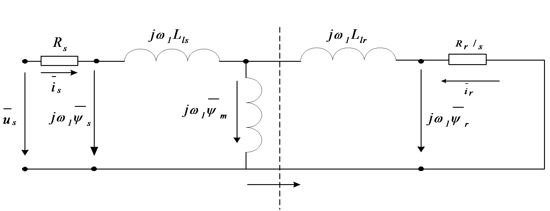
| (7.31) |

| (7.32) |

Based on the (7.31) and (7.32) equations the flux equivalent circuit is shown in Figure 7-8. The vectorial diagram of voltages and fluxes in a stationary case can be seen in Figure 7-9. According to the Figure 7-9, in synchronous speed co-ordinate system  , all the vectors are constant, and the voltage and rotor equations become
, (7.33)
| (7.34) |

7.3. Modified Equivalent Circuits
The equivalent circuits stemming from the flux equations normally use a per unit effective turn or reduction ratio. In this case the magnitudes in relative units are  . In many cases it is worth to choose a turn ratio which differs from the 1:1 ratio, because of the consistent simplifications in the motor equations. Let us introduce the fictive reduction factor a for the rotor quantities.
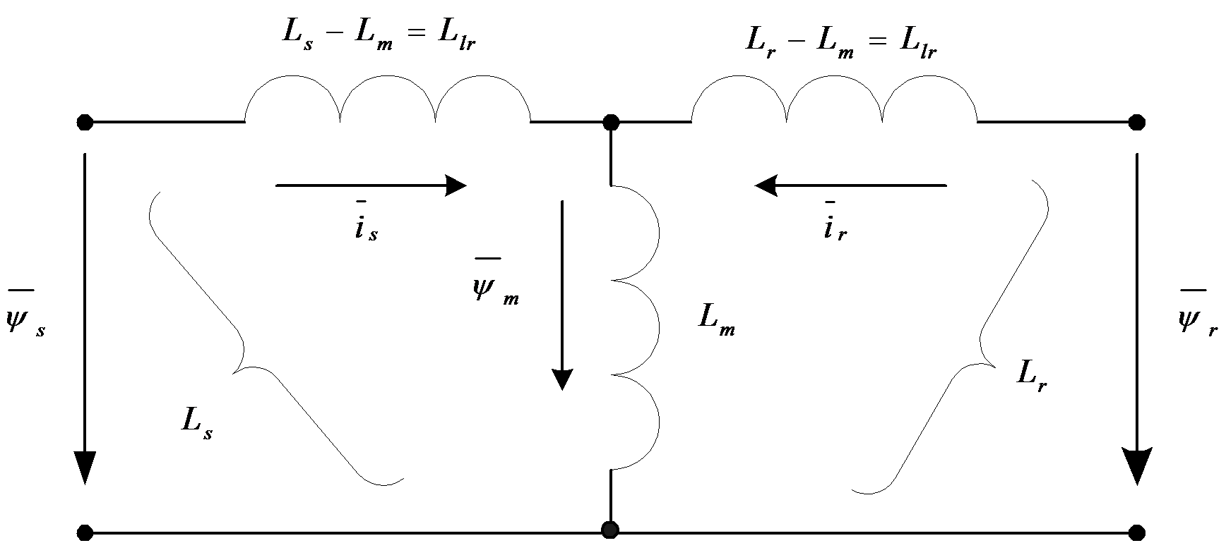

,  ,
,  ,
,  . In this case the flux equations (7.31) and (7.32) will be
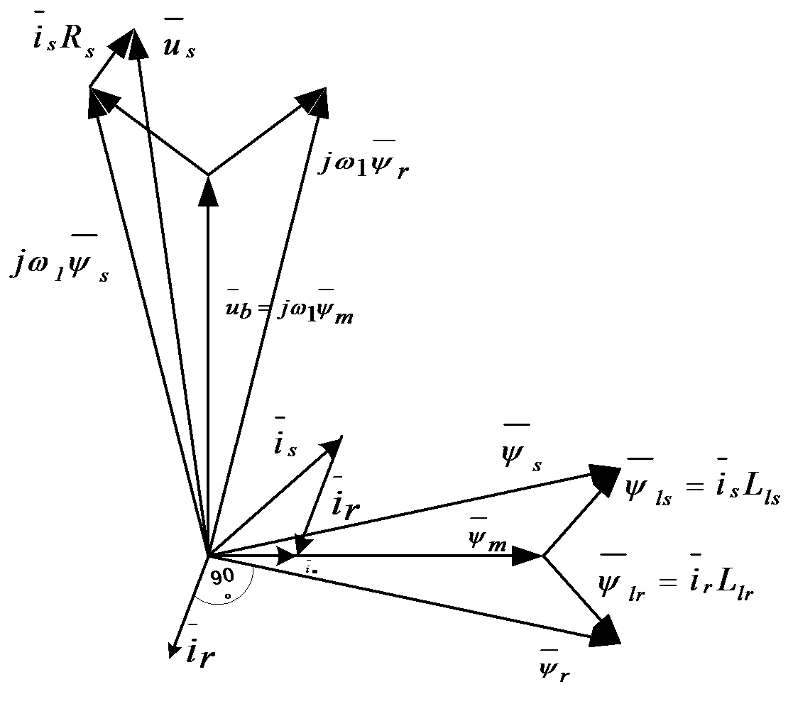
| (7.35) |
| (7.36) |
where  ,
,  ,
,  ,
,  . The reduction factor can be chosen in such a way that, after reduction, one of the reduced leakage factors becomes zero.
  , if
, if  ,
, 

 and
and  , if
, if 

 . If we use the above mentioned numbers for the inductance in the case of 1:1 reduction ratio, we get a1=2.5/2.5+0.11-0.4 and a2=2.5+0.1/2.51.04. Simplified flux equivalent circuits can be used in this case when the reduction ratio alters from 1:1, with a few percent. In Figure 710., and Figure 711. two simplified flux equivalent circuits are presented. Evaluating the fluxes marked by “*”,with the original inductance values (in the case of 1:1 reduction ratio), further simplification of the model is possible. There is obvious need to introduce the motor transient inductance
  , which is the resulting inductance from the primary site, neglecting the resistors and considering the secondary part in a short circuit. In the equivalent circuit (Figure 78.) according to fluxes, we can choose
  instead of
  :
:
| (7.37) |
| (7.38) |
| (7.39) |
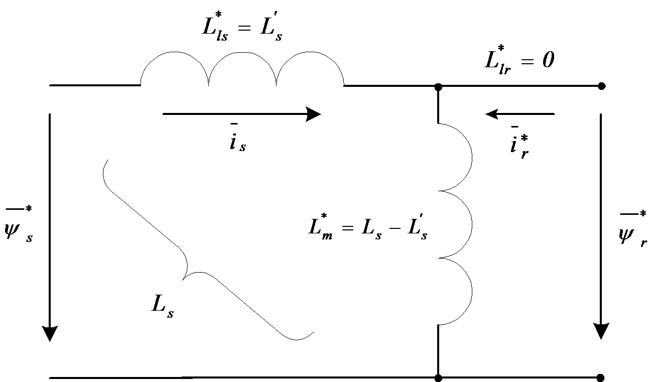
| (7.40) |
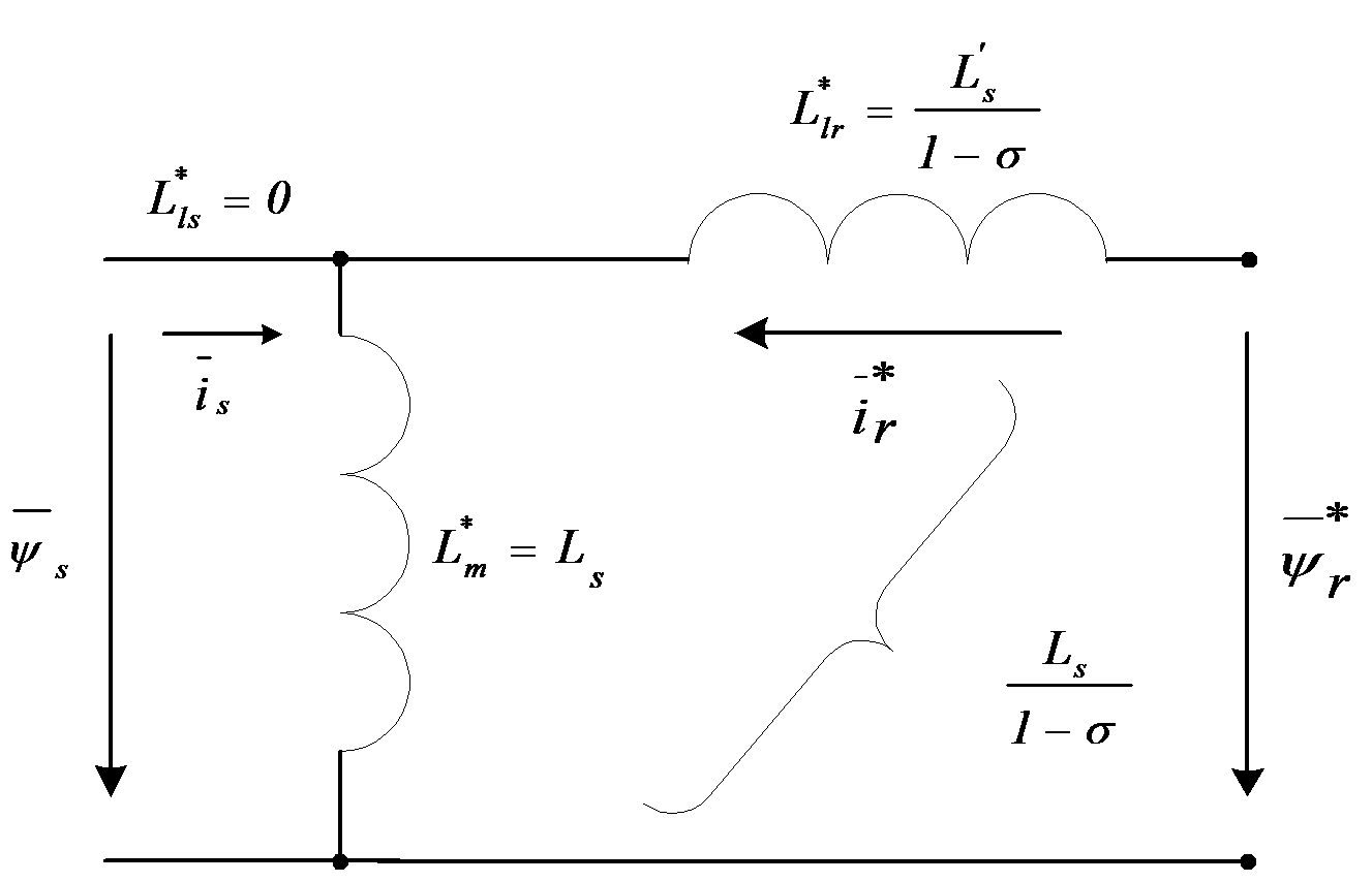
where is the resultant (total) leakage coefficient and k is the coupling coefficient. The  rotor transient inductance is the secondary resultant inductance, neglecting the resistors and considering a short circuit in the primer circuit. So calculating with
  we get
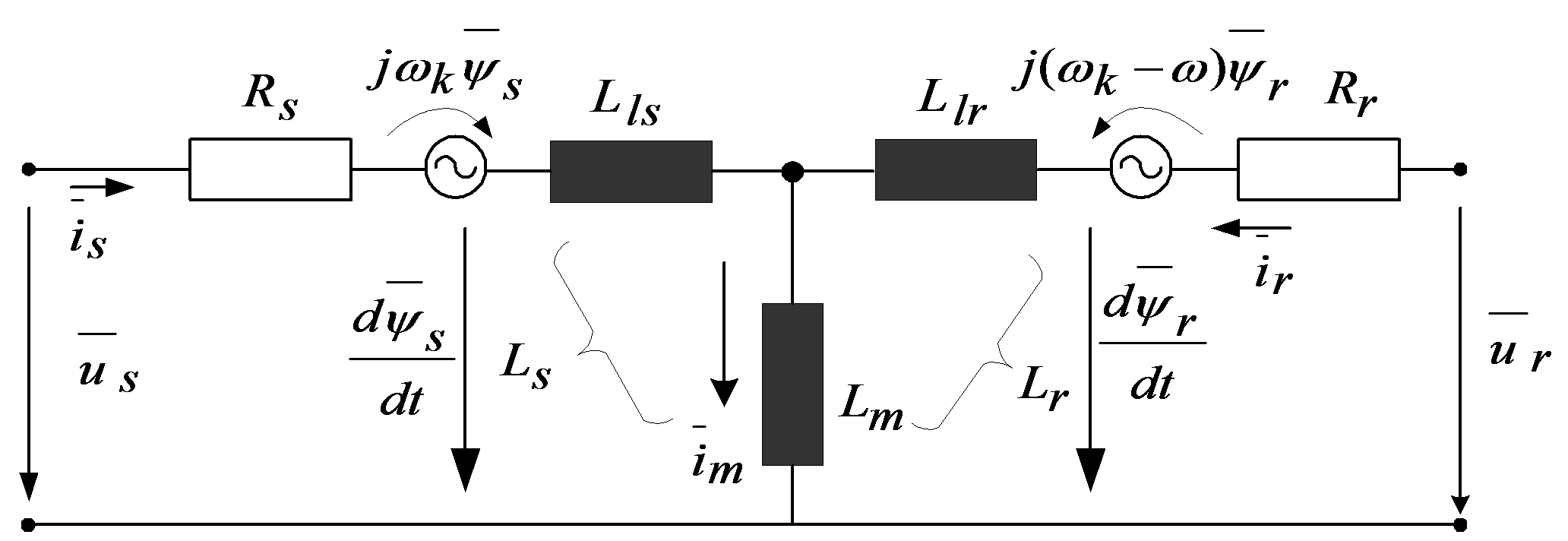
| (7.41) |
| (7.42) |
| (7.43) |

In case of Figure 7-10., we have
| (7.44) |

In case of Figure 7-11., we have
| (7.45) |
As it can be observed on the figures, the main field, in the case of the first figure, is  , while, in the case of the second figure, it is
  . Knowing the values of
  ,
,  or
or  , both equivalent circuits of Figure 710. or Figure 711. can be useful. It is evident that in this case the reduction must be effectuated also for the voltage equations, as follows:
| (7.46) |

| (7.47) |
This form matches the original equation, so if we choose the mode of reduction the “*” notation can be omitted. The Figure 7-12. presents the motor equivalent circuit, which is also valid for transient operation of the machines.
Taking the above statements into consideration, and regarding the modified equivalent circuits, for the purpose of further analysis, an equivalent circuit has been chosen, where the rotor leakage impedance has been included into the expression of the stator transient impedance. The new equivalent circuit can be seen in Figure 7-13. In this case, as we will see later on, the program calculates the voltages corresponding to the necessary current of the motor, instead of using a current control loop. Because the algorithm running time is less than the rotor time constant, the flux can be considered as constant. Consequently, the chosen equivalent circuit, where the rotor leakage impedance is properly included in the stator transient impedance (Ls'), is a good choice.
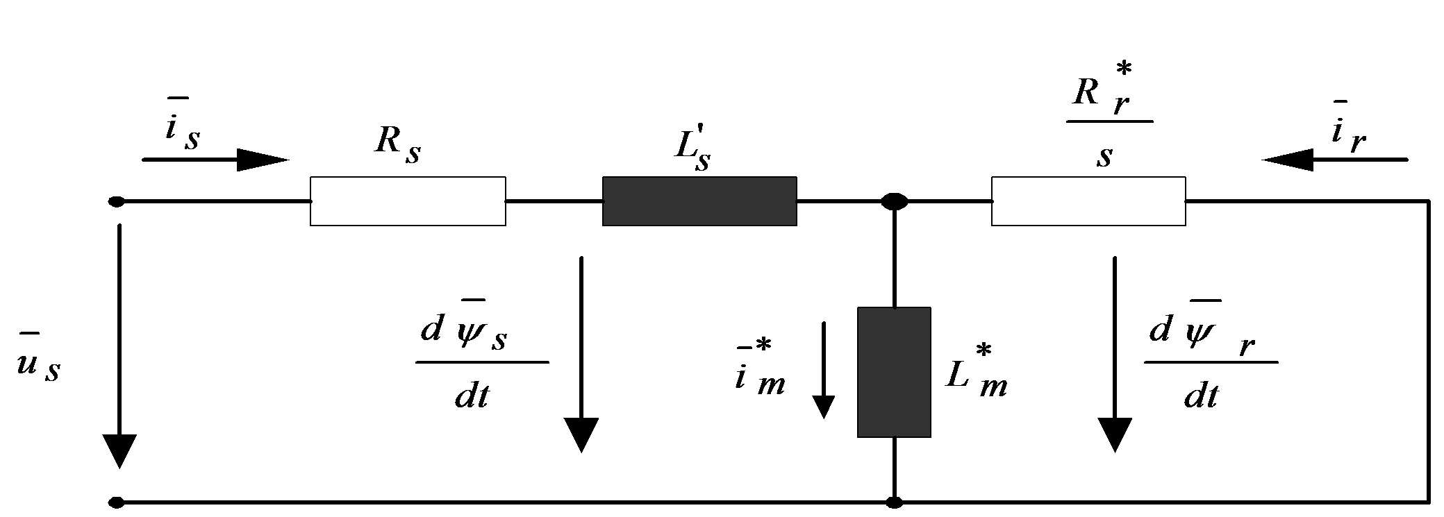
After reducing the motor's physical parameters and transforming the equations mathematically, the expression of the stator voltage vector equation will be as follows:
| (7.48) |
As we can see on the following pages, this equation will play a very important role in setting up the control structures, and also in applications.
7.4. Setting up the Model
Let us choose first a standstill co-ordinate system  , which means that the common co-ordinate system is a stationary one. Replacing the value
  in the general equations of the motor given by (7.20), (7.21), (7.22), and (7.23), the following vectorial voltage equations conclude:
| (7.49) |
| (7.50) |
Let us fix  and
and  as state variables. After the elimination of the terms
  and
and  from the above differential equation system, we get the following equations:
| (7.51) |

| (7.52) |
| (7.53) |
Solving the above equations according to the chosen state variables we get
| (7.54) |
| (7.55) |
For simplifying the above equations let us make the notation.
| (7.56) |
The has been defined in (7.40). Using again the complex representation of the vectors  and
and  , the model of the induction motor when
  are considered as state variables can be written in the following matrix form:
| (7.57) |
In same references when the two phase coordinate system does not rotate the quantities  are used instead of d,q quantities. So in the rest of the theses the when , components are used these refer to a stationary two phase coordinate system, when d,q components are used these will be the quantities in a special rotating two phase-system (field coordinates). The model of the induction motor will be described in field co-ordinates (in none of these models of the Asynchronous Motor do we take the mechanical losses into account), considering now the motion or cinematic equation of the motor, which is very important when we apply stochastic observers for the motor. As a basis, now again, the equations deduced in the previous paragraph, but with notations slightly changed as described also in [14], [15] will be used. This system of equations is nonlinear. The indices "r" and "s" mean rotor and stator, respectively:
| (7.58) |
| (7.59) |
| (7.60) |
, where  is the rotor angular velocity.(7.61)
The definition of the inductances in these equations and the total leakage factor is as follows:
| (7.62) |
where Lm is the main inductance of the motor,  and
and  are the resistances of the windings and Lls, Llr , are the leakage inductances of the stator and rotor respectively.
This model has been realized in SIMULINK for test and simulation purposes. See Figure 7-15. for the graphic realization. We will now define the model of the asynchronous motor in field co-ordinates. This will make it possible to implement the controller in field co-ordinates. Field orientation is described in detail in [16], and in the following sections. The basic principle is that we convert all values to the co-ordinate system of the magnetic field, decompose the stator current vector into a field generating and a torque generating ( and
and  ) component. At this moment the actual control becomes very simple. Since the program is designed so that the field weakening range will not be reached, the field generating component of the stator current voltage vector can be kept at a constant value to generate a necessary field, and control the torque generating component according to the speed. This means that the output of the speed controller is the reference for
  . We will eliminate the use of flux in the model, and we will use the magnetizing current instead. The connection between these two variables is the following:
| (7.63) |
where is the angle of the rotor magnetizing current vector with respect of the stationary axis. This quantity will play an important role in vector control when the special reference frame will be fixed to the rotor flux. The transformation between the systems will be done by the following transformation:
| (7.64) |
First, let us consider a brief overview of the state vectors (also called state phasors) represented in different co-ordinate systems as shown in Figure 7-14.
7.5. Stator Coordinates
Let us now switch to a Descartes coordinate system and fix it to the stator (, stationary reference frame). In this case the speed of the rotating coordinate system is  . Let us choose the stator current and the rotor flux to be the state variables. It means that we have to express these quantities from the general motor model described in equations (7.20)-(7.23). The resulted scalar model-equations are:
| (7.65) |

| (7.66) |

| (7.67) |
| (7.68) |
The rotor time constant is denoted by  .
.
These equations are now rewritten in a state space form with state variables isα, isβ, Ψrα and Ψrβ.
| (7.69) |
| (7.70) |
| (7.71) |
| (7.72) |

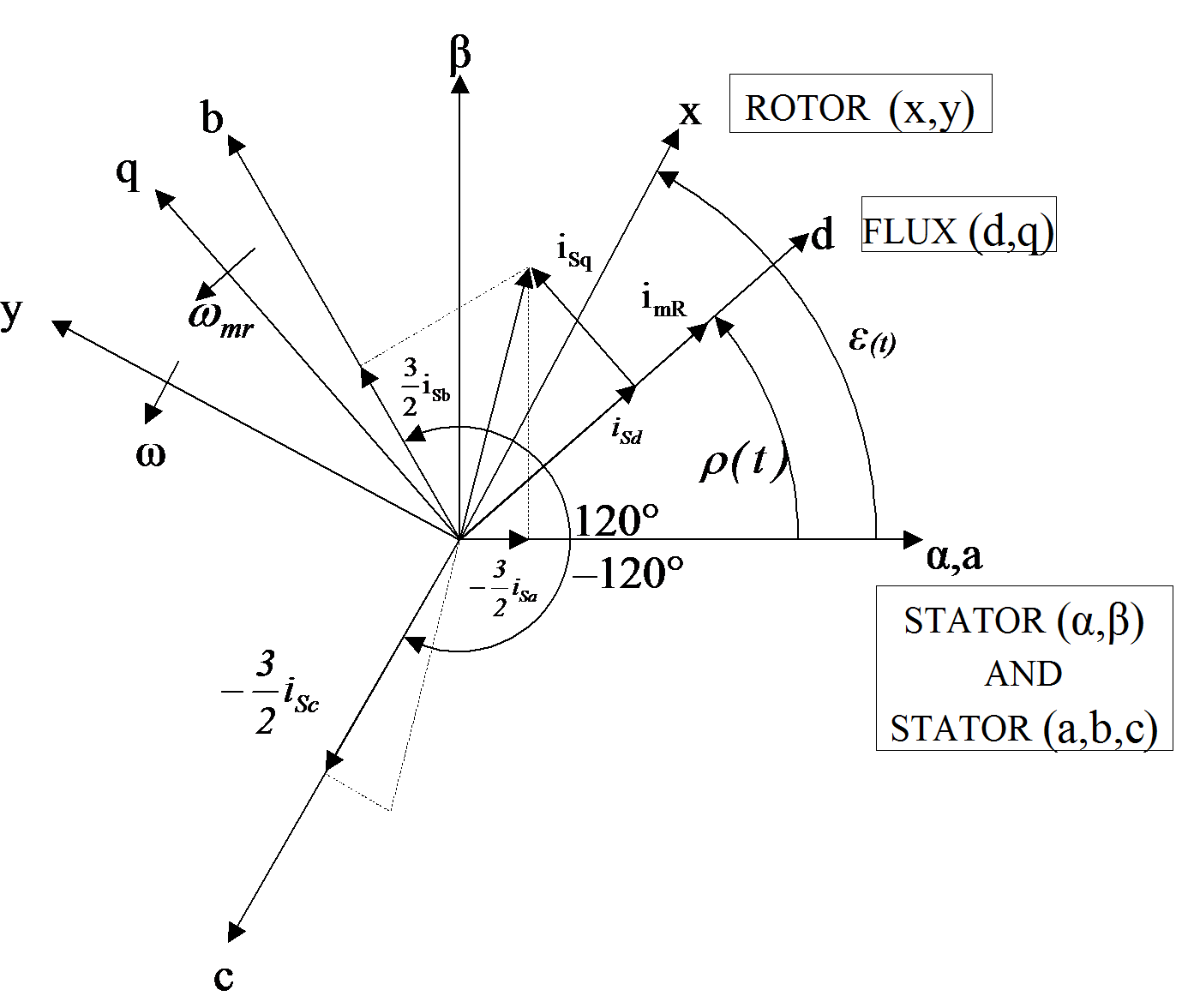
The stator time constant is denoted by  . The kinematic equations of the motor in stator coordinates are as follows:
| (7.73) |
| (7.74) |
| (7.75) |

where mL is the mechanical torque and p is the magnetic pole count.
7.6. Field Coordinates
Choosing the rotor flux as orientation quantity, that means all quantities are viewed from the rotor flux point of view, which are usually called field coordinates. The advantage of using this reference frame is that all quantities are constant in the steady state. The flux is now eliminated by introducing a new quantity called magnetizing current (rotor current cannot be measured) see eq. (7.63). The stator current (in field coordinates) and the magnetizing current are now chosen to be the state variables. The resulted scalar model-equations are:
| (7.76) |

| (7.77) |

| (7.78) |
| (7.79) |
Let us now rewrite these equations in a state space form where state variables iSd, iSq and imR are used. Notice that by introducing the magnetizing current we need only three state variables.
| (7.80) |
Where  , that is, the flux speed equals to the rotor speed plus the slip angular velocity of the rotor flux. The kinematic equations of the motor in field coordinates are:
| (7.81) |
The forms of equations remains unchanged in this coordinate system too. Equations presents the transformation matrices between the three-phase and the Descartes stationary coordinate systems, describes the connection between the stator and the field coordinates.
| (7.82) |
| (7.83) |
Figure 7-14. is a summary of the state vectors (also called state phasors) represented in different coordinate systems. Note that the rotor based variables are completely eliminated.
7.7. Model assumptions for the FOC method
Using the field oriented model of the motor, it has theoretically become possible to realize a control in field orientation, which makes it extremely easy to control speed by controlling  . However, our system of equations is nonlinear. We will eliminate this non-linearity by decoupling the nonlinear terms. This method has been described in [14], and detailed treatment is also given in [17]:
7.7.1. Decoupling of the Nonlinearity
We can see from (7.63), - that the model of the induction motor is nonlinear and time-variant. Let us now examine how nonlinearity is eliminated by decoupling the undesirable nonlinear and coupling terms.
| (7.84) |
| (7.85) |
| (7.86) |
| (7.87) |
We would like to control the speed. Let us recall . The torque is directly proportional to imr and to isq. Because Tr is large, imr cannot be used for a quick control. The leakage factor of iSq is small, that is why iSq can be used to control the torque and the speed. We get the best dynamic behaviour when imr is kept constant, therefore  can be assumed. This will remove the last non-linearity by making
  constant: Supposing that the main inductance Lm is time invariant, the rotor flux Ψr is kept constant, too. Under this assumption, using , , , and -(7.87) we get the following linear and decoupled model of the induction motor:
| (7.88) |
Where
| (7.89) |
Assuming that  is kept constant, KJ is also constant. In this case the system described by can be split into two independent parts, the direct (denoted by d) and the quadrature (denoted by q) subsystem:
| (7.90) |
| (7.91) |
After this it is possible to control the motor, provided that we are able to convert all values to field co-ordinates. This is made by the flux model (see the description later in the Simulink realization in Figure 7-21. and Figure 7-22.). The form of the flux model which has been realized here is based on [16], [18] and a Simulink realization done by dSPACE GmbH. After realizing the flux model control becomes possible. The first loop of the control is a controller for imr, which is in fact a controller for the rotor flux. There is a controller for isd, which will force the correct imr. The second loop begins with a controller for  , followed by a controller for isq, which will force the correct torque, and implicitly will realize the correct velocity. The overall control structure is shown in Figure 7-23. and Figure 7-24.
7.7.2. The Matlab/Simulink Model of the AC Motor
The model of the AC motor, which is sometimes called simply ASM = Asynchronous Motor, has been implemented in Simulink according to the equations as described in [16] and [14]. The actual model of the ASM can be seen in Figure 7-15. This model is based on the mathematical model described in [16]. However, it has been adapted to the requirements of Simulink. For the sake of simplicity, all vector variables have been substituted by scalar variables. The model is in stator and rotor co-ordinates. These equations have the advantage of an easy implementation, and great symmetry. The stator co-ordinates are indexed with S, the rotor co-ordinates with R, as before, and the indices  and a
and a  denote the two axes of the co-ordinate systems. The realized equations of the model presented in Figure 7-15. are the following:
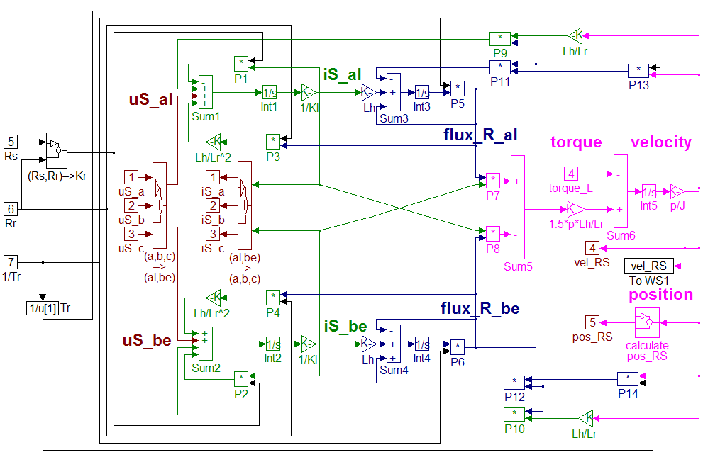
| (7.92) |
| (7.93) |
| (7.94) |
| (7.95) |
| (7.96) |
| (7.97) |
| (7.98) |

The basic functionality of the above model was tested with sine voltage signals excitation in open loop. The speed settled near the speed of the signals, that is, the rotor moved almost synchronously with the generated voltage vector. Then a torque was applied, which introduced a slip into the system. Since the voltages did not change, the speed of the rotor sank to a lower level. This chapter also describes the adaptation of the ASM (Asynchronous Motor) model for different kinds of algorithms, including sensorless control, too. The first step to design a Kalman filter, for example, is to have an appropriate model, which is used by the filter. For this purpose, we followed the method presented in [19] and derived the model, which was compared with the results of [14] and the results were the same. The model taken as a basis was the field oriented model of the motor based on [19], described by the equations presented in -. These equations can be formulated in such a form which is non-linear, but can be converted into a time-dependent matrix form. Let us see how to convert these equations:
| (7.99) |
This can be further modified by replacing  based on (7.106), and substituting
  by Ts. We get the following:
| (7.100) |

| (7.101) |
| (7.102) |
| (7.103) |

These equations can now be written in matrix form. Since we do not have a sensor for the load torque, it will be simply omitted, and regarded as a disturbance. Also note that the transformation matrix between the field and the stator is introduced to the equations, and so the input and output variables are in stator co-ordinates. This form is easier to handle in the case of the observing problem.
| (7.104) |
| (7.105) |
Note that in this model, and in all the following models, is part of the output vector. This does not mean that we measure it, but it must be estimated roughly, and this estimated value must be substituted into the Kalman filter where this output vector is needed. The substitution is made using the following formula:
| (7.106) |
For practical implementation we will need the model in discrete time, so let us consider the conversion to discrete time. Let us denote the system matrices of the continuous system with A, B and C, and those of the discrete system with Ad, Bd, and Cd. If we suppose that our sampling time is very short, as compared to the dynamics of the system (which is the case in most applications), we can generate the system with the following approximate equations (first order Taylor series, see [19]):
| (7.107) |
| (,7.108) |
| (7.109) |

With these, now we can present the system in discrete time.
| (7.110) |
| (7.111) |
This system is dependent on the values of  and
and  , which were regarded as known values until now. In [19], however, the Kalman filter is presented also as a substitute for the flux model, and the flux is observed as well. The first implementation does not follow this method, but it will be presented because further improvements may be based on it. The reason why a smaller model was chosen is that the dimension of the model is one of the most important factors determining the speed of calculation, and the reduction of a 6th order model into a 4th order one, which is relatively simple, can be done at a greater speed than the extraneous calculation of the flux model. To observe the flux, we must observe
  and
and  . This will be done by adding these to the system as new state variables. This increases the order of our system to 6. To add the new variables, we will assume that the sampling time is short enough for the speed of the flux to remain constant within the sampling period. That is, we can assume that
| (7.112) |

| (7.113) |
With these assumptions we can establish the new 6th order system, which can be the base of a Kalman filter, which observes the flux as well. For convenience the discrete-time model of the induction motor in a stationary reference frame is also presented which will serve again for observer application (7.114), where the speed of the rotor can be added as a state variable of the system. In the equation T is the sampling time and has to be not confused with the time constant of the stator and rotor.
| (7.114) |
| (7.115) |
| (7.116) |
7.8. Vector versus Scalar control
The field-oriented theory is the base of a special control method for induction motor drives. With this control method, induction motors can successfully replace expensive DC motors. Nowadays this method has become general in induction motor drives of high precision. The main advantages of induction motors are their simplicity and their price as well as their greater reliability, especially in harsh industrial environments. Induction motors require very complex control algorithms because there is no linear relationship between the stator current and either the torque or the flux. This means that, because of the transient states, it is difficult to control the speed of the torque until the motor reaches its new stationary state. Controlling the rotor flux, since it cannot be measured, but only computed can solve the problem. The purpose of the controller is to keep the amplitude of the rotor flux at a constant value so that only its direction is changed. The field-oriented theory offers a suitable method for optimally control of the induction motors. The complexity of the method is compensated by the advantages. Field-oriented control can be used in a wide range of industrial applications, thanks to the development of power electronic components and microprocessor systems. To have a basis for comparison, let us now introduce very shortly the most traditional scalar control.
7.8.1. Scalar Control
Scalar control means that variables are controlled only in magnitude and the feedback and command signals are proportional to DC quantities. With a scalar control method, we can only drive the stator frequency using a voltage or a current value as a command. Regarding the scalar methods known to control an induction motor, one assumes that by varying stator voltages in proportion with frequency, the torque is kept constant:
| (7.117) |

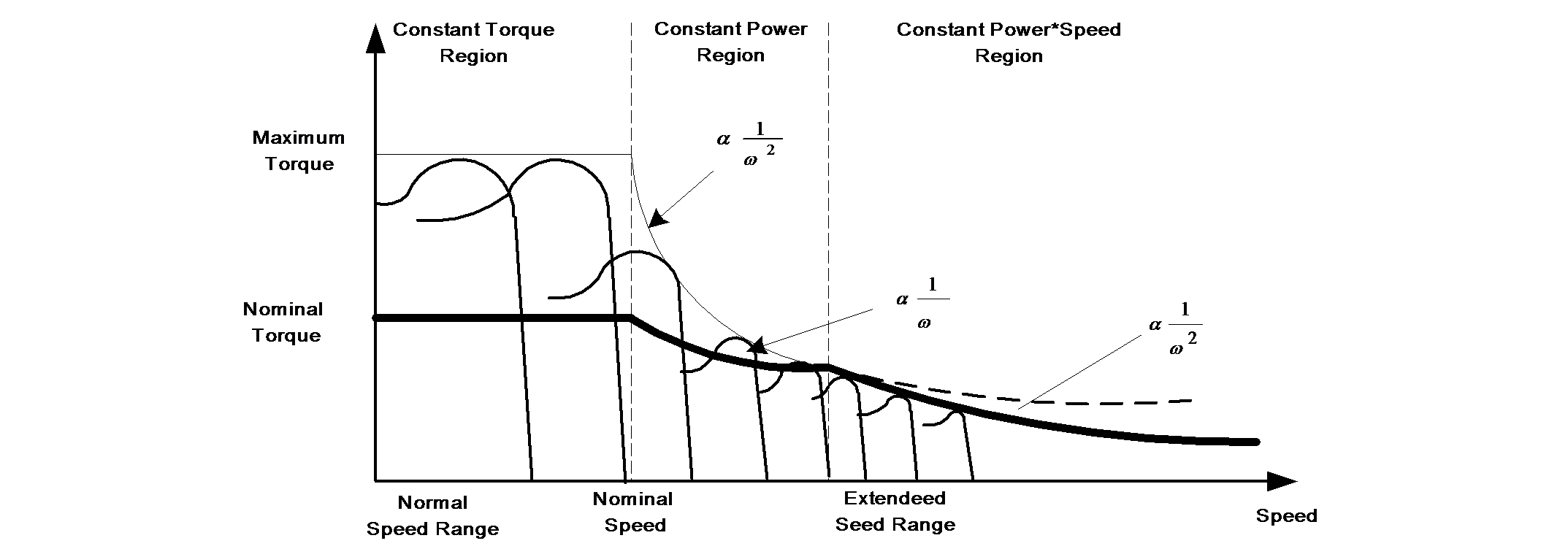
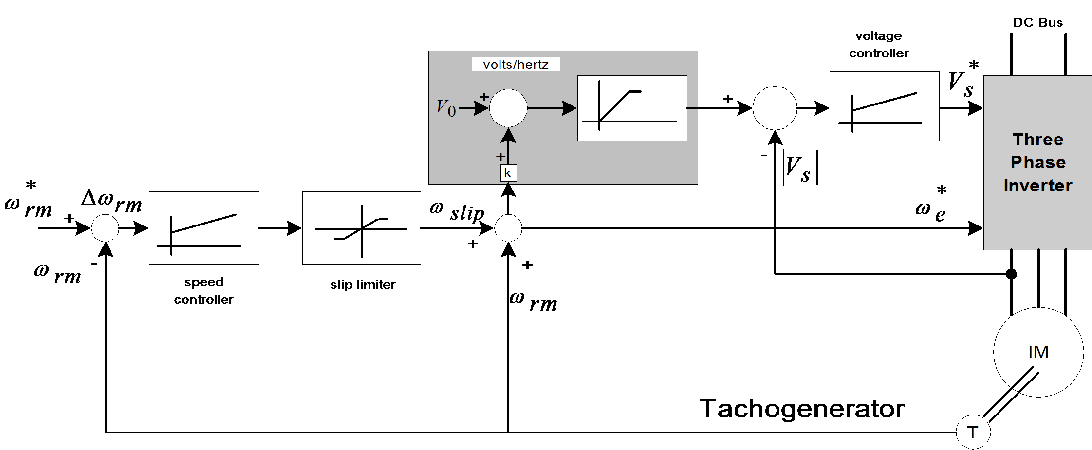
Figure 7-17. shows a closed-loop speed control scheme, which uses volts/hertz and slip regulation.
The controlled slip strategy is widely used because the induction machine’s input power factor and torque to stator current ratio can both be kept high, resulting in better utilization of the available inverter current. When air-gap flux and slip speed are both held constant, the torque developed will be the same, but the efficiency is not as good as that obtained with air-gap flux and slip held constant. When the slip is held constant, the slip speed will vary linearly with the excitation frequency and the slope of the torque-speed curve on the synchronous speed side will decrease with the excitation frequency. These control methods have been well studied in the literature and it is not the subject of this thesis to give a more analytical insight into this field. Rather, we will turn now to the presentation of the more important vector control principle and the associated questions in AC motor control based on this principle.
7.8.2. Vector Control
Vector control is referring not only to the magnitude but also to the phase of these variables. Matrices and vectors are used to represent control quantities. This method takes into consideration not only successive steady states but also real mathematical equations that describe the motor itself. The control results obtained have a better dynamic for torque variations in a wider speed range. The space phasor theory is a method to handle the equations. Though the induction motor has a very simple structure, its mathematical model is complex, due to the coupling factors to be applied to a large number of variables, and to the non-linearities. Field Oriented Control (FOC) offers a solution to circumvent the need to solve high order equations and to achieve an efficient control with high dynamic. This approach requires more calculations than a standard U/f control scheme. This can be solved by the use of a calculation unit included in a Digital Signal Processor (DSP), and has the following advantages:
full motor torque capability at low speed,
better dynamic behavior,
higher efficiency for each operation point in a wide speed range,
decoupled control of torque and flux,
short term overload capability, four-quadrant operation.
7.8.2.1. The FOC Algorithm Structure
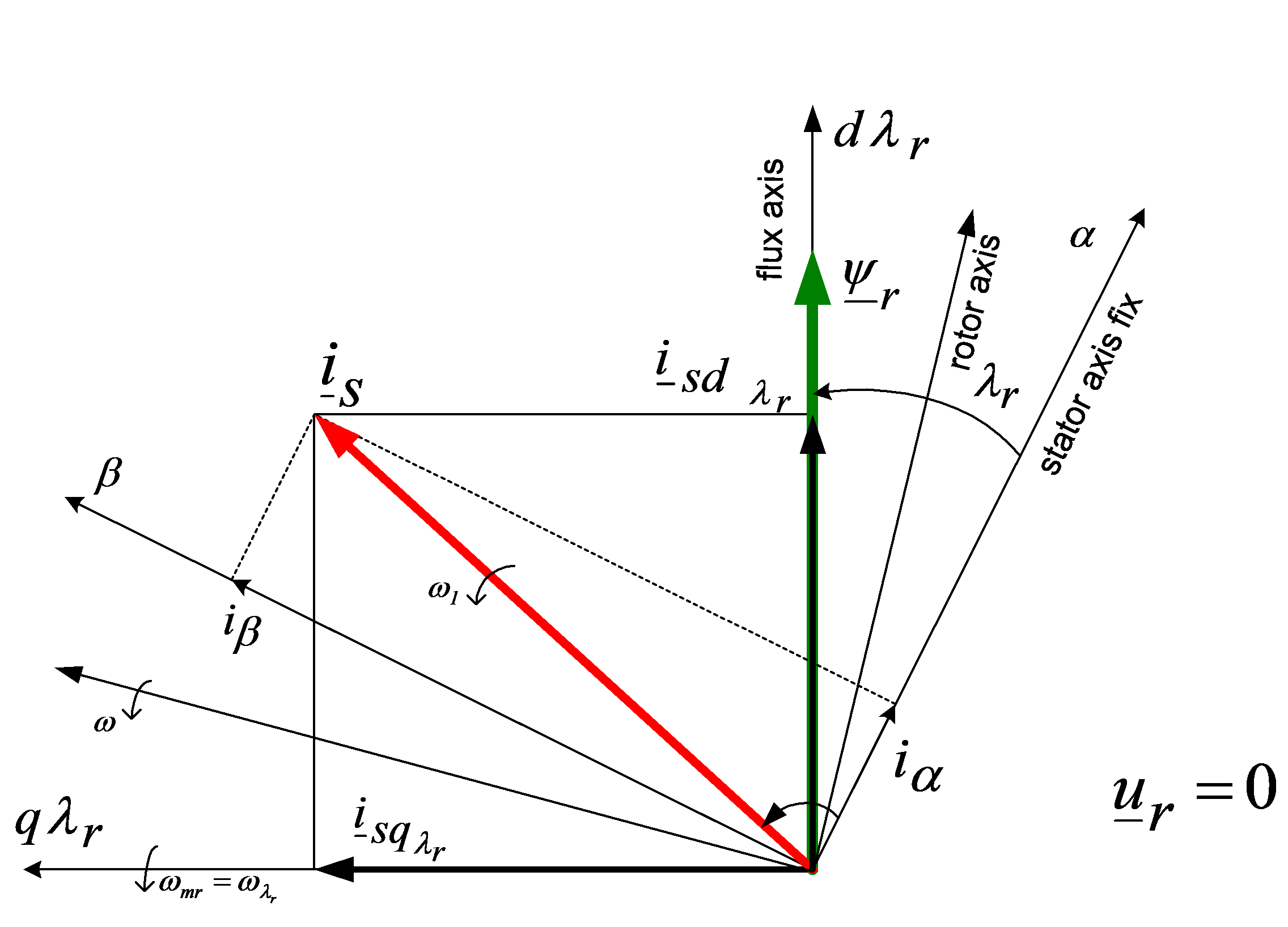
FOC consists of controlling the components of the motor stator currents, represented by a vector, in a rotating reference frame d,q aligned with the rotor flux. The vector control system requires the dynamic model equations of the induction motor and returns the instantaneous currents and voltages in order to calculate and control the variables. Stator current and flux space vectors in the d,q rotating reference frame and the relationship of that with the , stationary reference frame can be seen in Figure 7-18. The control of induction machines must take place in an orthogonal reference frame that rotates with rotor flux angular velocity ( ) in such a way that the d
 axes coincide with the instantaneous position of the rotor flux
  . In this case the torque expression has just one term, a current multiplied by one flux. The orthogonal components of the fluxes will be zero. The current in the torque expression will not be other than the projection of stator current vector to the q
 axes, and can be characterized as the active current. The stator current projection to the d
 axes gives the magnetizing current of the motor. In this way the induction motor can be controlled by two separate loops: one for the reactive current (flux) and one for the active current (torque or speed), like a separately excited DC motor. The flux identification procedure defines the type of the control system.
There are very simple cases where the orientation flux and its position are determined by measurement. When this is not possible, in the majority of cases, the orientation quantities are determined by using the mathematical model of the induction machine expressed in the orthogonal co-ordinate system. A complex control system can define the orientation quantities in one co-ordinate system and control the motor to another. In Figure 7-19. the space phasor diagram of the induction machine with short circuited rotor windings is proposed. The most often used method is the one with rotor-resultant-flux orientation, because of the simple structure of the control loops and easy command variable calculation. The space phasor of the stator current is split into two components, which become control variables. Vector rotation techniques are used to transform three phase axes into rotating two-phase "d-q" axes. This two-phase rotation technique greatly simplifies the analysis, making it equivalent to analyzing separately excited DC motors, because in this case there are two independently controllable currents: the field current and the armature current. In a two-phase system  and
and  represent the stator current in the stationary reference frame where the axes of the two-phase system exactly match the “a” axis. To control field and torque independently, we must use the moving "d-q" co-ordinate system, rotated at the synchronous speed with respect to the stationary reference frame. Projecting
  onto "d-q" yields the components
  and
and  . To control these quantities the stator current vector must be oriented to "d-q", where
  is the orientation angle. Let us omit the presentation of co-ordinate transformations related to the vector control strategy because they have been well described in the literature. We only summarize here the transformations that must be effectuated:
(a,b,c)(,) is the Clarke transformation, which outputs a two-co-ordinate time-variant system, and
(,)(d,q) is the Park transformation, which outputs a two co-ordinate time-invariant system.
This is the most important transformation in FOC. In fact, this projection modifies a two phase orthogonal system in a (d,q) rotating reference system.
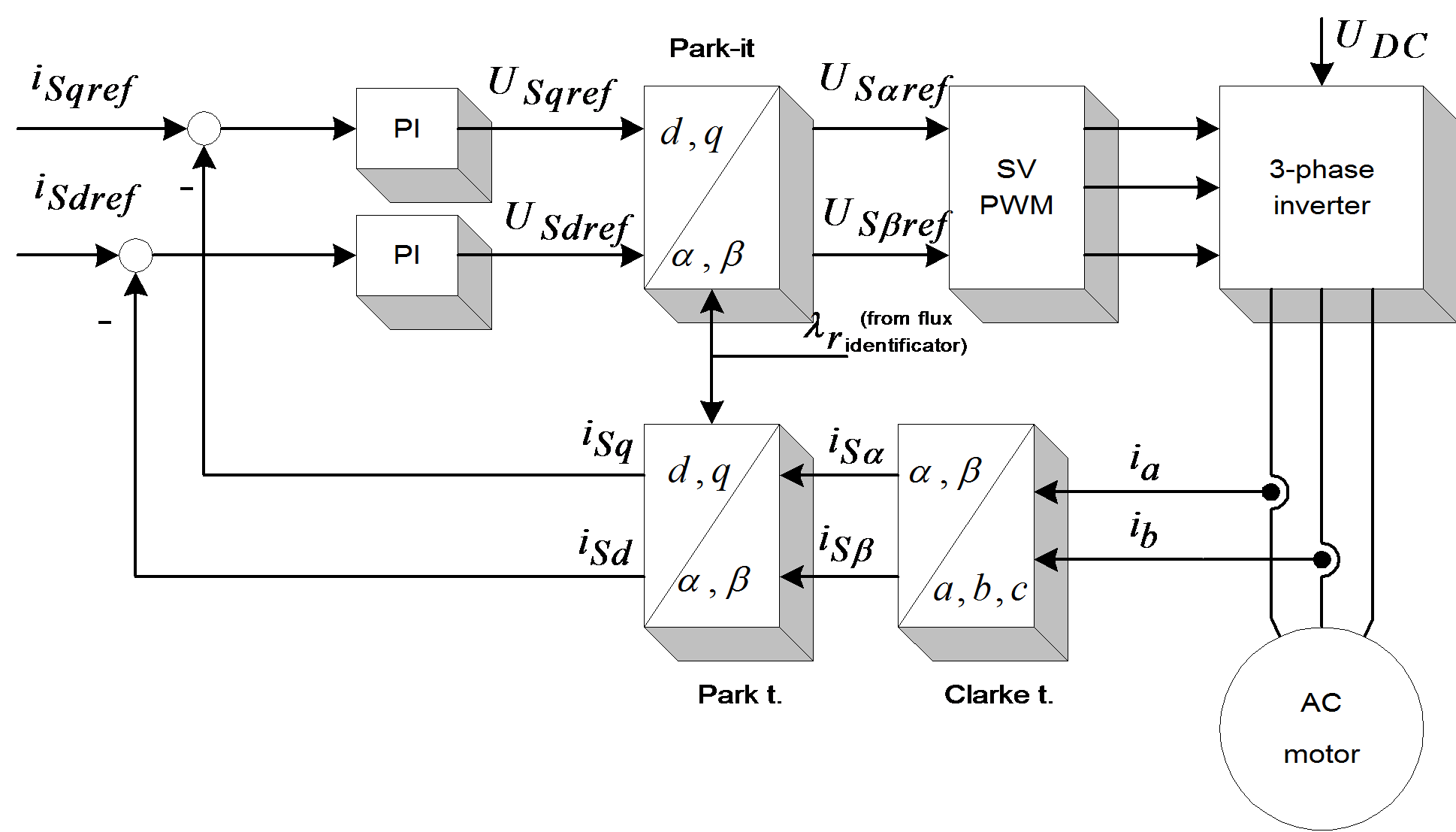
The (d,q) (,) projection is the inverse Park transformation.
The outputs of this block are the components of the reference vector, which is the voltage space vector to be applied to the motor phases. Figure 7-20. summarizes the basic scheme of torque control with FOC. Two motor phase currents are measured, which feed the Clarke transformation module. The outputs of this projection are designated is and is. These two components of the stator current are the inputs of the Park transformation that gives the current in the d,q rotating reference frame. The isd and isq components are compared to the references (isd)ref (flux reference) and (isq)ref (torque reference). At this point, this control structure shows an interesting advantage: it can be used to control either synchronous or induction machines by simply changing the flux reference and obtaining the rotor flux position. As in the case of synchronous permanent magnet motors, the rotor flux is fixed (determined by the magnets) there is no need to create one. Hence, when controlling a PMSM, (isd)ref should be set at zero. As induction motors need rotor flux creation in order to operate, the flux reference must not be zero. This conventionally solves one of the major drawbacks of the “classic” control structures: the transferability from asynchronous to synchronous drives. The torque command (isq)ref could be the output of the speed regulator when we use a speed FOC. The outputs of the current regulators (usd)ref and (usq)ref are applied to the inverse Park transformation block. The outputs of this projection are (us)ref and (us)ref, which are the components of the stator vector voltage in the (,) stationary orthogonal reference frame. These are the inputs of the Space Vector PWM. The outputs of this block are the signals that drive the inverter. It is worth to remark that both the Park and the inverse Park transformation need the rotor flux position. Obtaining this rotor flux position depends on the AC machine’s type (synchronous or asynchronous). Some considerations with regards to rotor flux position for motors of the asynchronous type are the following. If the controlling method is based on the field-orientation principle, the identification of the oriented quantities is of crucial importance. This includes the calculation or prediction of the position and magnitude of the chosen flux, the control of the active and reactive currents in the d-q reference frame, and the recovery of these quantities in a,b,c quantities, which can control the motor through a static type frequency converter. The structure of the control system and the type of the frequency converter must be taken into consideration when making the important decision on which flux is to be used in orientation. The control systems differ not only in this respect, that is, which flux is used in orientation, but also in the identification procedure. There are very simple cases, when the orientation flux and its position are determined by measuring (direct vector control). When this is not possible, as in the majority of cases, the orientation quantities are determined by using the mathematical model of the induction machine (indirect vector control), written in the orthogonal co-ordinate system. This latter co-ordinate system can be oriented after another phasor (not only the flux phasor), in the scope of operation, with a simpler mathematical model.
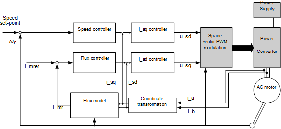
Consequently, if a complex control system can define the orientation quantities in one co-ordinate system, and control the motor to another, the field-orientation cannot be used by itself. For this reason, the vector control terminology is appropriate for this system, rather than that of field-orientation. Another classification methodology can also be adapted to a field-oriented control system, based on the determination of the field-orientation quantities, when the parameters are identified on-line. This method means real-time identification and tracing of process quantities like the resistance of the rotor and the changes of the rotor’s time constant. This method is applicable to such systems where the torque has a low changing rate. A more efficient method is where parameter identification is determined off-line, with the help of a mathematical model of the motor, the method of previously testing the machine, is applicable on a large operation scale.
The electric torque of an AC induction motor can be described by the interaction between the rotor currents and the flux wave resulting from the stator current induction. Since the rotor currents cannot be measured with cage motors, this current is replaced by an equivalent quantity described in a rotating co-ordinate system called d,q following the rotor flux. The instantaneous flux angle  is calculated by the motor flux model, which will be given later. isd and isq, the stator current components in the d,q frame, are obtained directly from ia, ib and ic, the fixed co-ordinate stator phase currents, with the Park transformation:
| (7.118) |
In steady-state conditions the stator current is defined in the above mentioned rotating system is considered constant, as well as the magnetizing current imr representing the rotor flux, isq being equivalent to the motor torque. isd is linked to imr [16] and [18] with the following equation:
| (7.119) |
where  is the rotor time constant. This system together with the angle transformations, changes the induction motor into a machine very similar to a DC motor where imr corresponds to the DC motor’s main flux, and isq to the armature current. The field-oriented control method achieves the best dynamic behavior, whereby the lead and disturbance behavior can be improved with shorter control cycle times. The field oriented control method is a de facto standard to control an induction motor in adjustable speed drive applications with quickly changing load as well as reference speeds. Its advantage is that by transforming measurable stator variables into a system based on field co-ordinates the complexity of the system can be enormously reduced. As a result, a relatively simple control method, very similar to that of a separately exited DC motor, can be applied. The role of the DSP in such a system is to translate the stator variables (currents and angles) into a flux model as well as to compare the values with the reference values and update the PI controllers. After back transformation from field to stator co-ordinates, the output voltage will be impressed to the machine with a symmetric or asymmetric PWM, whereby the pulse pattern is computed on-line by the DSP or a hardware generated space vector method. In some systems the position is measured by an encoder. This extra cost can be avoided by implementing an observer model, or, in particular cases, a Kalman filter. These algorithms are complex and, therefore, require a fast processor. A fixed-point DSP is able to perform the above controls with short cycle times. Let us repeat here the basic equations of field orientation, which are deduced in [18]. Substituting the rotor current in the rotor voltage equation and considering the magnetizing current equal to the rotor flux divided by main the inductance, we can express the d-q components of the stator current phasor as follows:
| (7.120) |
The d component of the stator current vector is influenced by the rotor-flux amplitude variation, and the q component by the relative speed between the rotor-flux space-phasor and the rotor’s spatial position. Looking at the equation (7.120), we can notice that whenever the rotor-flux magnitude is not constant, the d component of the stator current contains a new element, proportional to this flux variation, and respectively, to the magnetizing current (delay element). The electromagnetic air-gap torque can be calculated from the flux-oriented variables as follows:
| (7.121) |
If the variables are all rotor-flux-oriented, the following expressions can be obtained:
| (7.122) |
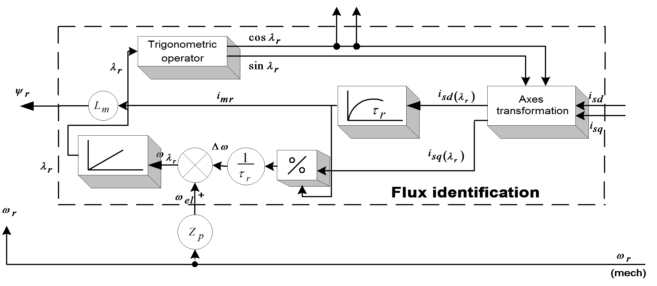
The rotor-flux-oriented components of the stator current space phasor  can serve for the control of rotor flux and the machine torque, respectively. Let us take a look now at the calculation of the orientation quantities based on the above-deducted equations. As the input stator components must be oriented and the orientation variables appear only at the output of this block, internal calculations to determine the trigonometric functions are needed. The structural scheme of the flux identification is given in Figure 7-21. The stator current components are field-oriented. The two non-linear differential equations prove to be stable under all operating conditions and their continuous on-line solution on a DSP does not raise problems. It is more advantageous to use stator currents instead of voltages, due to their reduced harmonic content. This is the reason why at stator frequencies lower than 100 Hz, a sampling time of 1ms and a 10-bit resolution A/D converter are permitted. The stator resistance and leakage inductance have no influence on the orientation-field calculation, as the feedback loop is independent of the stator voltage model. Of real interest are the rotor parameters, especially the time constant
  , influenced by the rotor resistance (varying with the temperature), and the iron-core saturation. The torque calculation is also dependent on Lm and on the rotor leakage coefficient
  . In order to achieve higher speeds, higher than the nominal values, the stator frequency has to be increased. In high frequencies the stator resistance can be neglected. If the flux magnitude variation is also neglected, the voltage equation becomes very simple:
  , where
  is the synchronous frequency. It is obvious that if the flux is kept constant, the limit voltage of the converter is reached at a certain stator frequency. Thus the flux must be reduced if further speed increase is needed. Under such operating conditions, in the so-called field weakening region, the stator voltage is kept approximately constant at its maximum.
7.9. Summary
When the rotor is short circuited and if the rotor flux magnitude is constant then the rotor current vector is perpendicular to the flux phasor direction. In the equation (7.123) there is summarized the two cases of rotor flux identification are summarized. First, when the rotor flux magnitude is kept at a constant value, and, in the second case, it can change. In the latter case a time lag appears in the equation of the flux generation component of the stator current vector.
| (7.123) |
where
| (.7.124) |
The reactive current is influenced by the rotor flux amplitude variation, and the active one by the relative speed between the rotor-flux space phasor and the rotor’s spatial position. Comparing the above two equations, it can be noticed that whenever the rotor-flux amplitude is not constant, the reactive component of the stator current contains a new element, proportional to this flux variation and to the magnetizing current variation, respectively.
7.9.1. The Matlab/Simulink Model of the Field Oriented Control
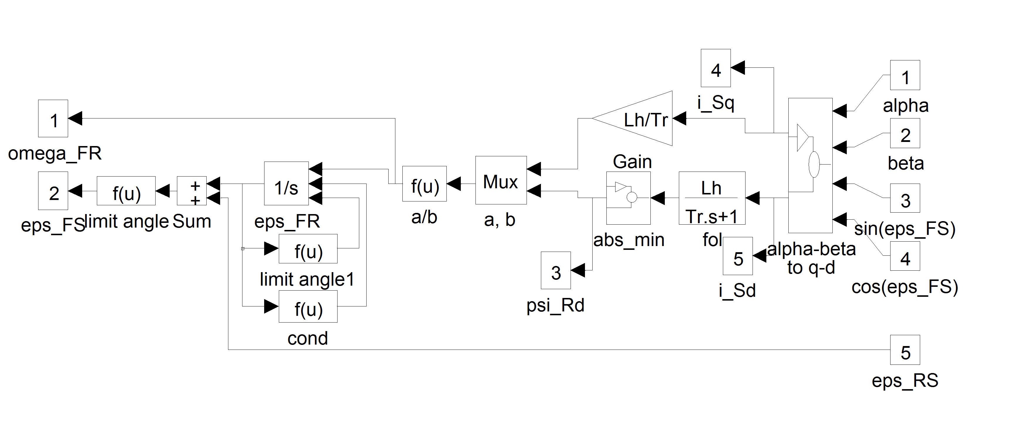
Let us give an overview from the point of view of simulation, on how the FOC can be implemented in Matlab/Simulink graphical development system. The differential equations treated in [16], [14], and [18] were taken into account. The usage of symbols was taken from the dSpace realization, to avoid possible misunderstanding. For the complete controller, the controlling parameters described in [15] were adapted. A slight modification to the structure of the theoretical flux model was effectuated. The flux model can be seen in Figure 7-22. Before carrying out the division by “psiRd” ( ), we have to make sure that its value is not zero, otherwise an infinite value gets into the system, which, in turn, causes all further calculations to "blow up". To make sure that this does not happen, we must "part"
  from zero by a small value. This task is done by the block "abs min". This block sets psi_offset as a minimal absolute value for
 . This means, that either
  <psi_offset or
  >psi_offset must be true. The value of psi_offset should be set to a small value, so that psi_offset<<psi_Rd_ref, where psi_Rd_ref is the reference, which is in our case a constant value. This is in fact a modification, which is implicitly included in the software, since in the software a division by 0 is saturated to the maximal or the minimal value of the fractional. The sine and cosine values of the transformation angle eps_Rd (
 ) are given twice: once for transformation, and once for inverse transformation. Avoiding this by calculating sine and cosine values only once, and using these values directly for both directions of calculation, gave results to a much faster working flux model. Let us show now the whole control system in Figure 7-24., and the FOC part of it in Figure 7-28.
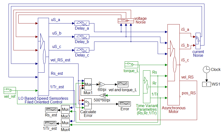
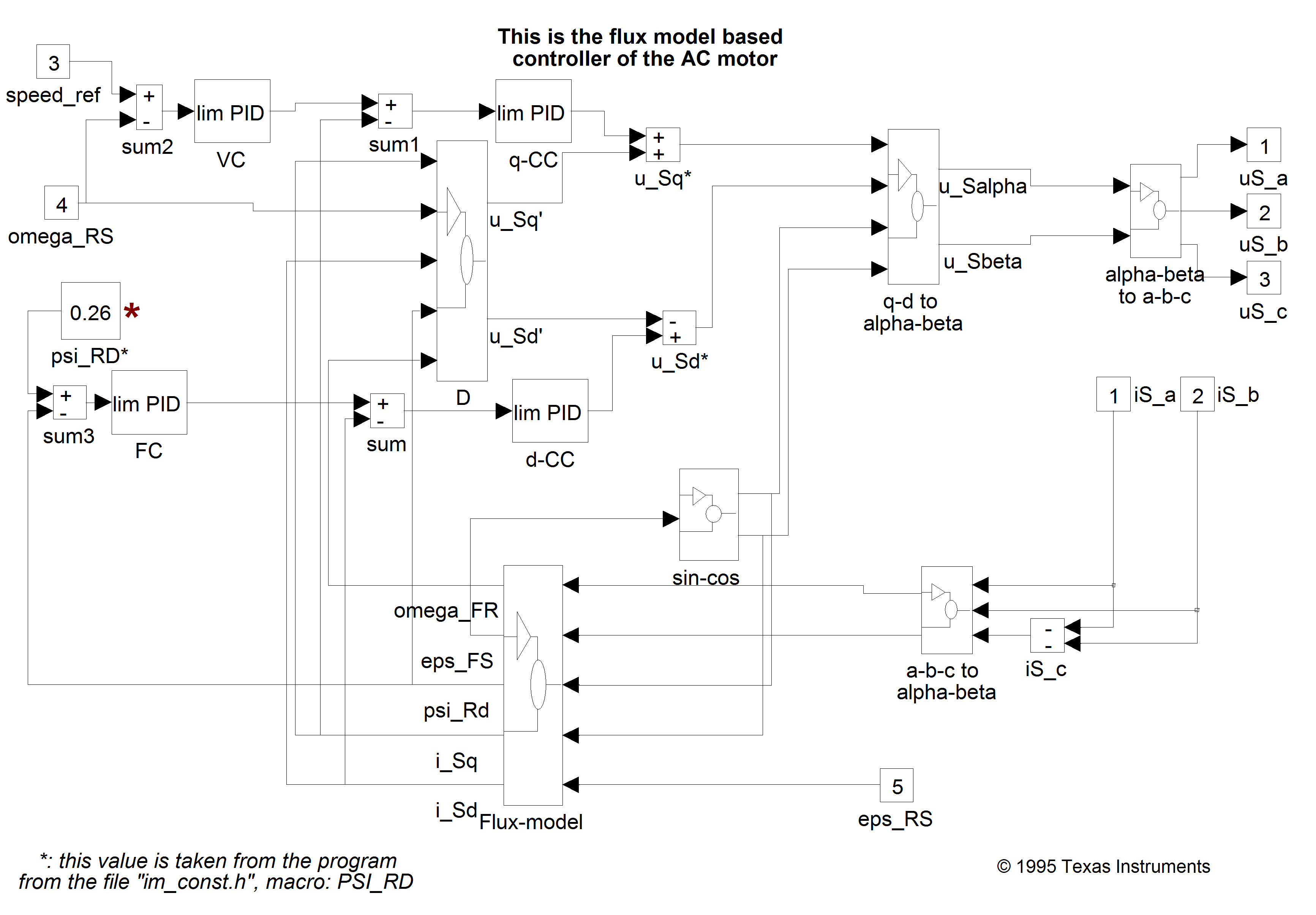
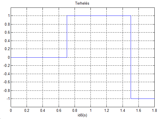
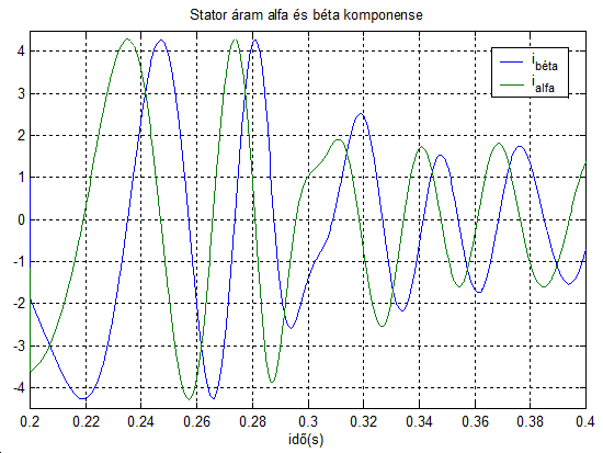
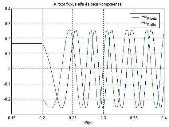
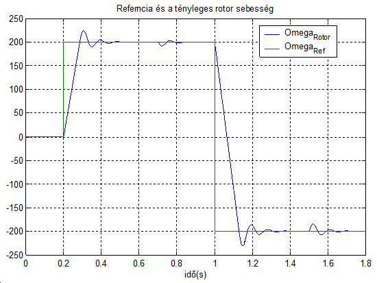
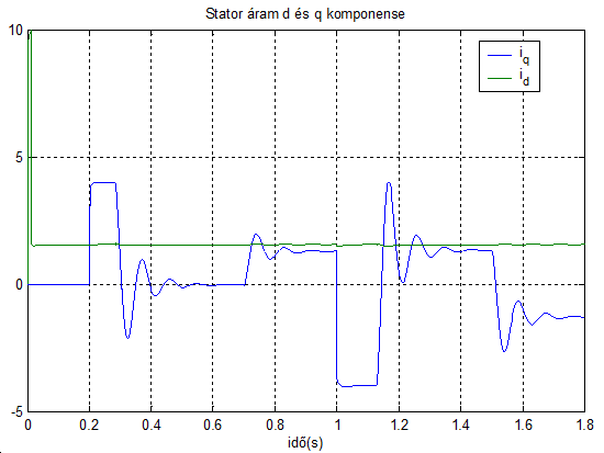
Chapter 8. Sensorless Control with Speed Estimators
8.1. Sensorless FOC Techniquess
In the case of induction motors, field oriented control (FOC), as compared to other control strategies, has great advantages. However, FOC requires the measurement of the speed, which may be technically unrealisable or extremely expensive. As a consequence, there is a strong interest in the FOC without any speed sensors. During the last five years several sensorless schemes have been proposed in the professional literature to identify the rotor speed by voltage and current measurements only [20]. In general, there is a trade-off between control performance and the the simplicity of implementation. Consequently, it is not possible to select the “best” general sensorless scheme [21]. The main objective of this chapter is to give an overview of the most important methods used in sensorless control of AC drives, to analyse them, and to compare a few of them with the traditional speed sensor-based methods. Bearing in mind the huge implementation efforts in the field of such kinds of applications, this chapter will focus on the simulation of the methods. Let us now review the basic concepts of the available field oriented sensorless techniques. This summary is mainly based on [21] and [20].
Speed Estimators (SE).
Model Reference Adaptive Systems (MRAS).
Luenberger Speed Observers (LSO).
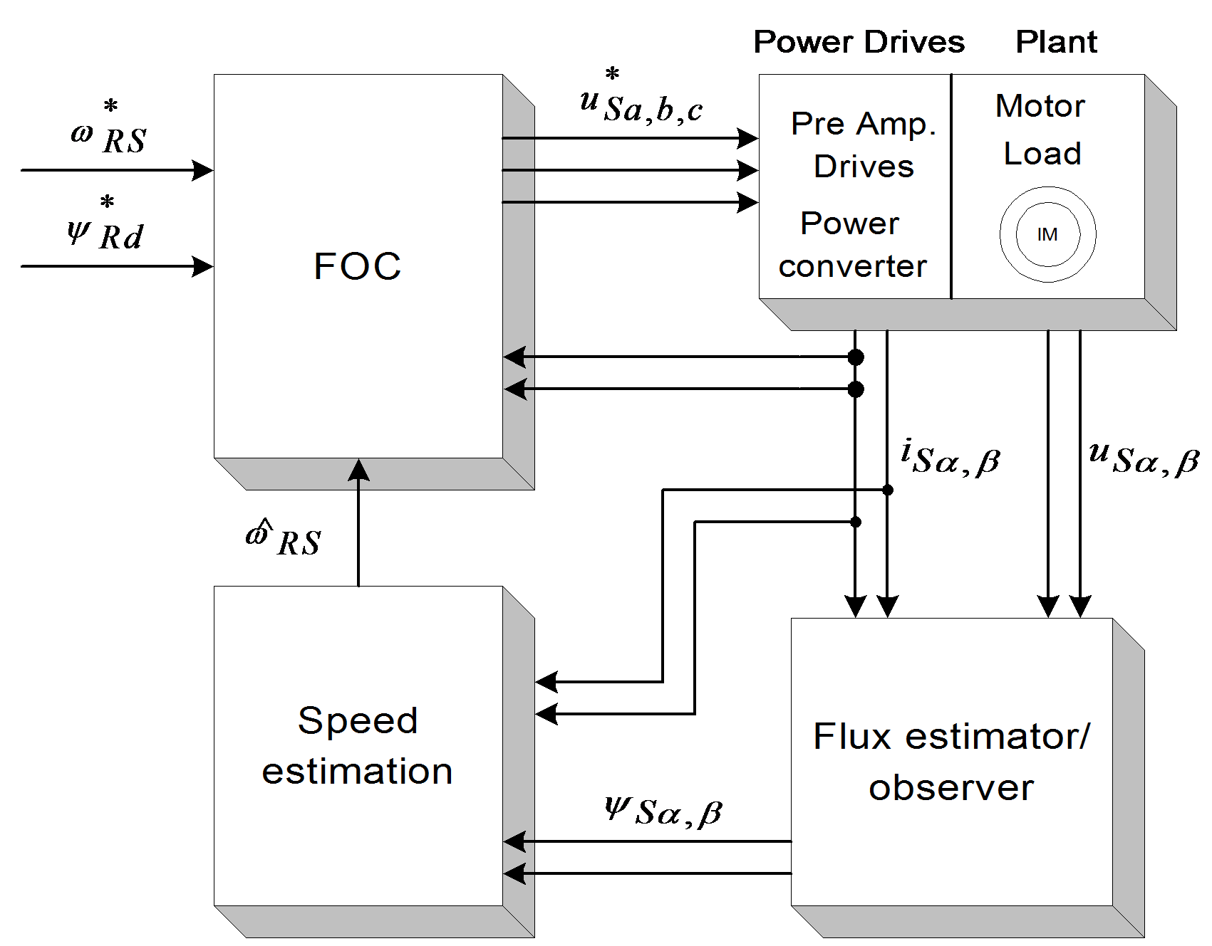
Speed estimators use measured stator currents and estimated or observed stator (or rotor) flux to estimate the speed. In most cases the rotor speed  is calculated as the difference between the synchronous pulsation
  and the slip pulsation
  :
:
| (8.1) |
Notice that the derivative of the flux is present, which means that the input voltages directly influence the estimated speed. The general model of this technique is shown in Figure 81. No feedback exists in the controlling cycle.
Model Reference Adaptive Systems are based on the comparison of the output of two estimators: one is the reference model, the other is the adjustable model. A suitable adaptation algorithm calculates the rotor speed from the output error. There is a feedback in the controlling cycle because the adjustable model uses the rotor speed. MRAS methods differ from each other in the output quantity q used for error calculation (see Figure 82.). The adaptation mechanism is the same for all model reference strategies:
| (.8.2) |

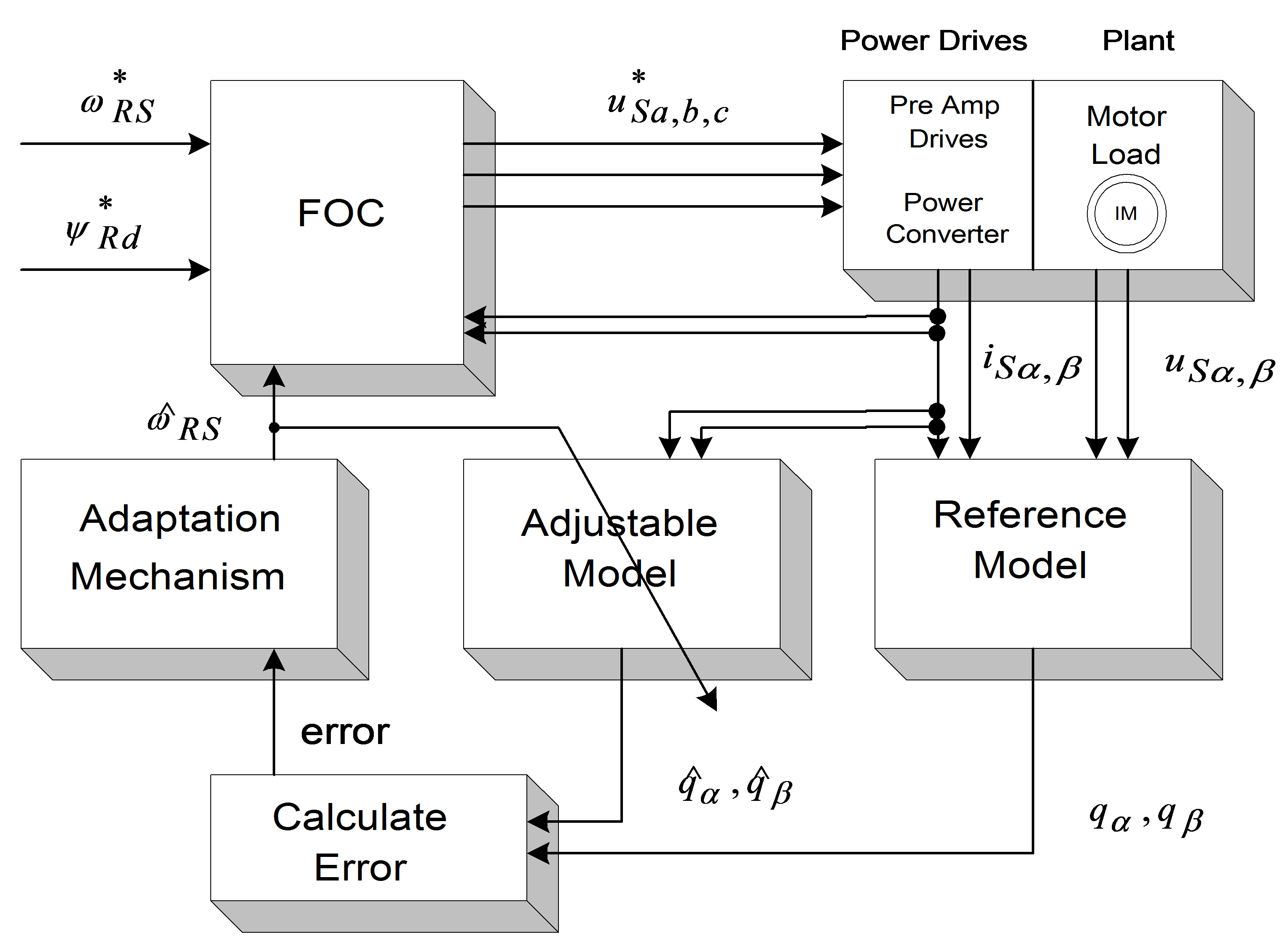
Luenberger Observer (LO) techniques are based on the fact that the rotor flux and the stator current are estimated by a deterministic (Luenberger) observer, and the rotor speed is calculated with an adaptive scheme using the stator current error and the estimated flux. If the rotor speed is included in the state variables of the observer, the scheme differs from the previous one. This is called the Extended Luenberger Observer (ELO). The two schemes are shown in Figure 8-3. and Figure 8-4. In terms of classification, these techniques are similar to the model reference adaptive methods if the motor is treated as the reference system, and the observer as the adjustable model.
The blockdiagram of the Kalman Filter based method is the same as that in the case of the Luenberger observer. The difference between them is the observer itself. The Kalman filter is a statistically optimum observer if the covariance matrices of the various noises are known. It means that the Kalman filter directly cares for the effects of the disturbance noises in- and outside the system. The errors in the parameters will also be handled as noise. A great difference in computation time exists between the Kalman filter and the Luenberger observer. In the case of the Kalman filter techniques, the observer gain matrix has to be computed in each controlling cycle. That is, many matrix operations and matrix inversions are required, resulting in a problem when implementing it in real-time. Generally speaking, the Kalman filter was developed for stochastic systems, and the Luenberger observer is, in fact, its deterministic case.
After reviewing the main ideas of the sensorless techniques, we would like to compare their performance, in order to select one of them for adaptation in the field oriented reference frame. In [21], this comparison is performed on the basis of the following set of criteria:
response time to load change steps,
low speed operation,
steady state error,
computation time,
parameter sensitivity,
noise sensitivity.
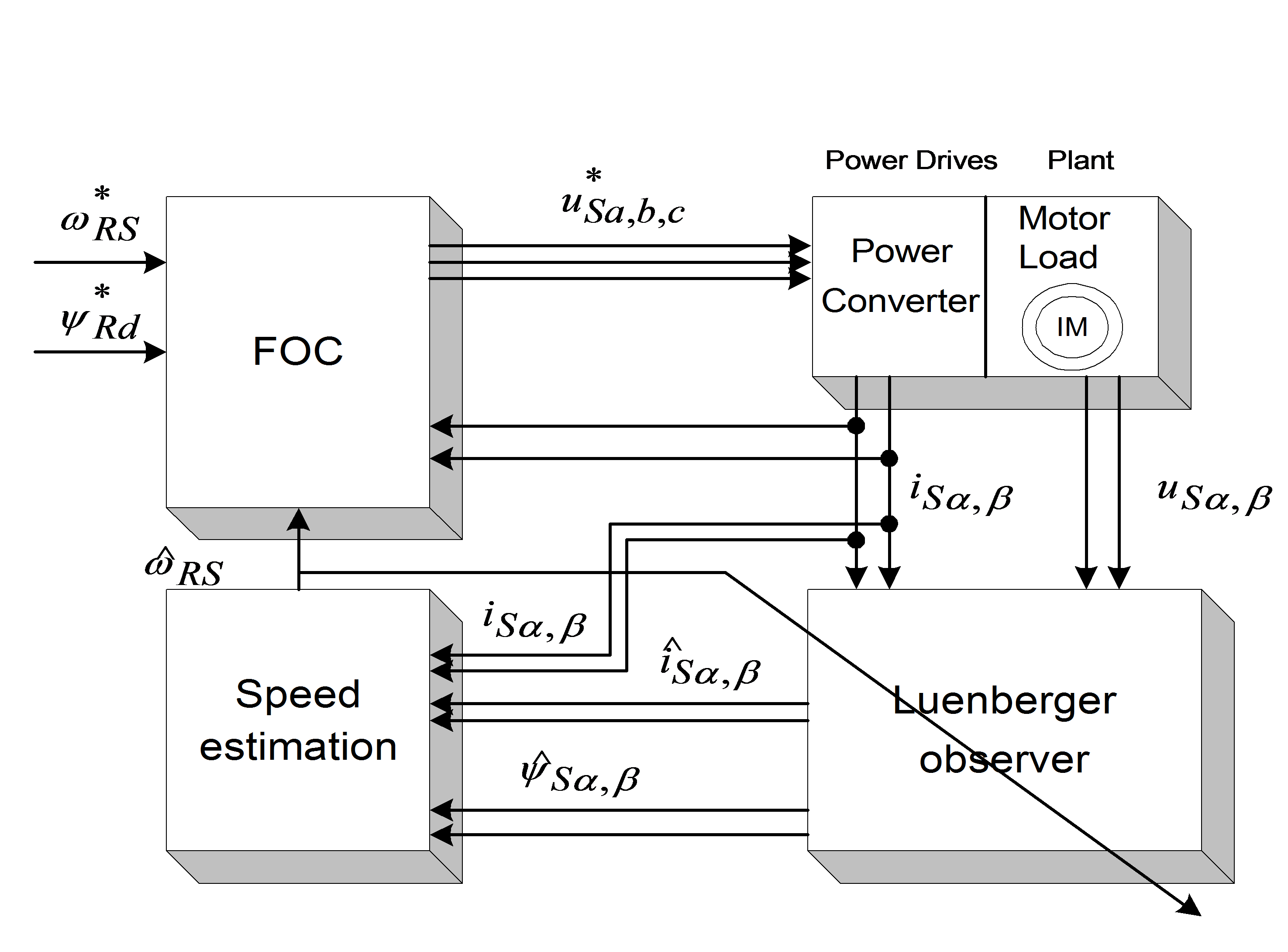
The problem for SE, MRAS, and KFT is that a trade-off exists between the good disturbance rejection and the short settling time when setting the speed PI gains. This problem does not occur in the case of LSO. SE, LSO, and KFT may work at very low speed (at e.g., at 20 rpm), while there is a minimum speed (about 100 rpm) for MRAS. SE and MRAS have a small steady state error when the motor is loaded [21]. KF algorithms contain many matrix operations, which causes problems when they are implemented on a DSP system. This problem does not exist at SE, MRAS and LO. When rotor resistance is detuned, LO seems to give the best result, and LE, MRAS, and KFT work similarly. The only stochastic system-based scheme, KFT gives an outstanding result when measurement and process noises are present. Our main specifications are to have a good dynamic behaviour at low frequencies, and a computational complexity as small as possible. EKF seems to give the best behaviour with respect to the criteria taken the most often into consideration, and is better in the case of measurement and process noises, however, it requires high processor capacity.
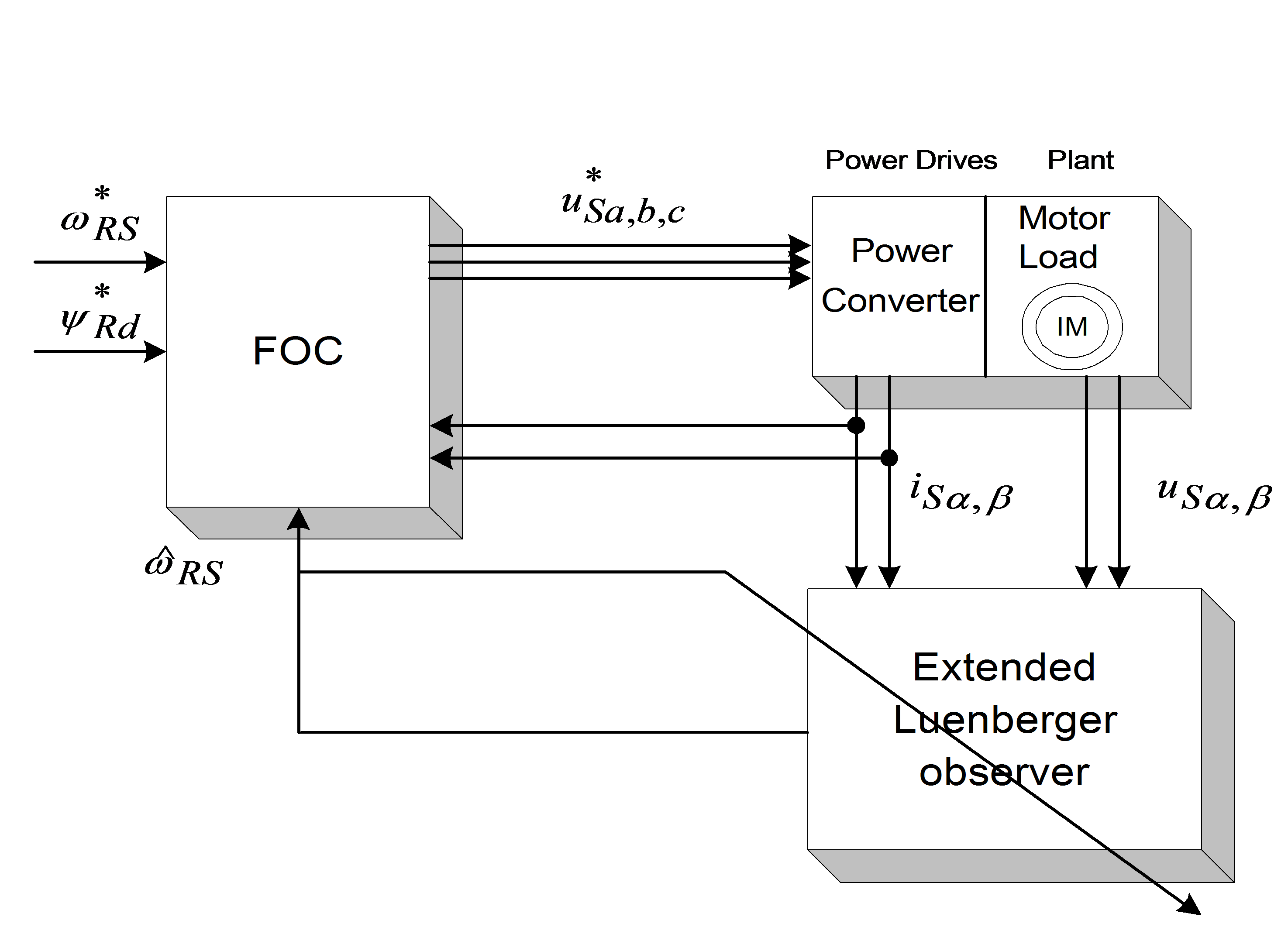
According to all these considerations, EKF has been selected for deeper analysis
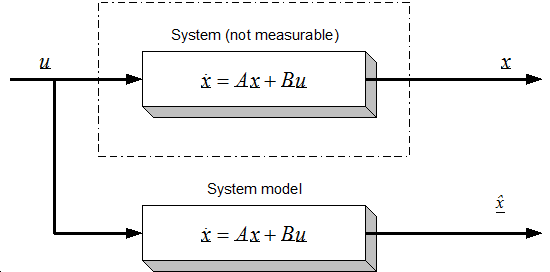
8.2. Observers’ Basics
Let us first formulate the problem of observers. Let us take a system which has some internal states, these state variables are normally not measurable, so we usually measure only substitute variables. If we want to know these internal state variables for some reason, for example, we want to be able to control them, then we have to calculate them. It is not always possible to calculate these variables directly from the measured outputs. Let us consider a system with the following form, which is actually the so-called the ‘state space form’. (Note that all symbols that denote matrices or vectors are underlined).

 ,(8.3)
| (,8.4) |

where u and y are the input and the output vectors and x is the state vector. A, B, and C are the system, input and output matrices. We measure the inputs and the outputs, but in most cases the states cannot be measured directly. If we need the value of a state variable (for example we want to control this state), we have to compute it from the measured quantities. In the case of asynchronous motors, we measure the currents and the voltages. We would like to control the speed of the rotor without any sensor (speed measurement means extra cost, may be technically impossible, etc.), that is, we would like to compute it from the measurements of the currents and of the voltages. It should be noted that the calculation of the states is not always possible (state observability), it depends on the system model [22]. An observer is used to determine the value of the states of a system. The general model of the state observer is shown in Figure 8.6 in the case of the LO, and Figure 8.5. in general case, for example, where  denotes the estimated state vector, L is the observer gain matrix, and a suitable way has to be chosen to make the output error r converge to zero. With a very simple approach we can realize a system that runs parallel to the real system, and calculates the state vector, as shown in Figure 85. This is based on the quite reasonable assumption that we know the input values of the system. This approach, however, does not take into account that the starting condition of the system is unknown, which is true in practically every case. This cause the state variable vector of the system model to be different from that of the real system. The problem can be overcome by using the principle that the estimated output vector is calculated based on the estimated state vector,
| (,8.5) |

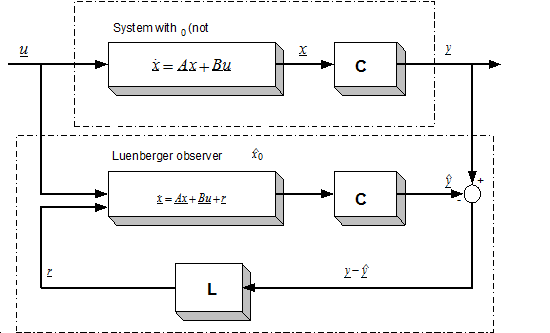
which may then be compared with the measured output vector. The difference will be used to correct the state vector of the system model. This is called the Luenberger Observer, and it can be seen in Figure 8.6. Now we can set up the state equation of the Luenberger Observer as follows:
| (.8.6) |
Now we can ask how the matrix L must be set in order to make the error go to zero. Setting up a state equation for the error as follows does this:
| (,8.7) |

where
| (.8.8) |

If we now transpose the matrix of the error differential equation, we get a form which is very similar to a controller structure:
| (.8.9) |
The effectiveness of such an observer greatly depends on the exact setting of the parameters, and on the exact measurement of the output vector. In the case of a real system, none of these criteria can be taken for granted. In the event of relatively great disturbances in the measurement, great parameter differences, or internal noises in the system, the Luenberger observer (as a deterministic case) cannot work anymore and we have to turn to the Kalman filter. Let us analyze the basics and the theory of the Kalman filter a little bit more because it is more important for our investigations, and its practical importance is much higher than that of a deterministic case.
8.3. The Kalman Filter Approach
The system we have considered up to now uses a sensor to measure the speed of the rotor. In many cases it is impossible to use sensors for speed measurement because it is either technically impossible or extremely expensive. As an example, we can mention the pumps used in oilrigs to pump out the oil. These have to work under the surface of the sea, sometimes at depths of 50 meters, and getting the speed measurement data up to the surface means extra cables, which is extremely expensive. It is clear that in such applications the most vulnerable part of the drives is the sensor. Cutting down the number of sensors and measurement cables provides a major cost reduction. Lately, there have been many proposals addressing this problem, and it has turned out that speed can be calculated from the measured current and voltage values of the AC motor. Some of these proposals are open loop solutions, which give some estimation of speed, but these solutions normally have a large error. For better results we need an observer or a filter, an estimator. The Kalman Filter has a good dynamic behavior, disturbance resistance, and it can work even in a standstill position. See [23] for a comparison of the performances of an observer, a Kalman Filter (KF) and an Extended Kalman Filter (EKF). Implementing a filter is a very complex problem, and it requires the model of the AC motor to be calculated in real time. Also, the Filter equations must be calculated, which normally means many matrix multiplication and one matrix inversion. Nevertheless, a processor with high calculation performance can fulfill these requirements. DSPs are especially well suited for this purpose, because of their good calculation-performance/price ratio. In low cost applications fixed point DSPs are desirable. The solution chosen by us is a Kalman filter, which is a statistically optimum observer (see exact details in [24]) if the statistical characteristics of the various noise elements are known. For the implementation of the Kalman Filter we need a much greater calculating capacity than that of the first generation C14 DSP, so at least a C50 DSP must be chosen to realize the field oriented control. This makes things more complicated of course, since the variables have to be scaled, which would be unnecessary with a floating-point processor. The Kalman filter is a special observer, which provides optimum filtering of the noises in measurement and inside the system if the covariance matrices of these noises are known. So let us first see what a stochastic estimator is.
8.4. Mathematical Background of Kalman Filters
When sampling the continuous-time and the discrete-time models of a system, it is very important to obtain the discrete time model of a plant or actuator, and, when needed, to apply an estimator or an observer to the system. A general state space model has the following equations in the continuous case:
| (8.10) |
The calculation of the transfer function with Laplace transformation: Executing Laplace transformation of equations (8.10) we gain the following equations:
| (.8.11) |
Rearranging equation (8.11) we get
| (.8.12) |
Then the transfer function of the system is
| (.8.13) |
Solving the state equation of the system by Laplace transformation:
For the inverse transformation we need the inverse of the term  . Let us first express this term in a geometrical series and we will see that in this case we can more easily effectuate the inverse transformation:
| (.8.14) |
Applying the inverse Laplace transformation to the terms in the series we will get an infinite series, which is the Taylor series of  around 0:
| (.8.15) |
The inverse Laplace transformation of equations (8.12) gives the solution for the state equations as follows:
| (.8.16) |
8.4.1. Let us now descretize the continuous system:
We use the above treated continuous model for deducing the discrete model. The system is usually discretized by an A/D converter which can be considered as a zero order hold system. Using the notations t=tk+1, t0=tk , we get the following equation:
| (,8.17) |
where  and T is the sampling period.
Let us introduce a new notation

,
and a new variable  , according to which
.
Introducing the above notations to (8.17) we get
| (.8.18) |
The value of u is equal to the value of u(k) because of the ZOH. The value of  is constant, so both of them can be brought out from the integral:
| (.8.19) |
After this the integral can be calculated or evaluated easily:
| (.8.20) |
From (8.19) and (8.20) we get the state space equation of the discrete-time system:
| (.8.21) |
The equation written in a matrix form is:
| (,8.22) |
Where
| (.8.23) |
From here on, we will work with discrete systems, so, for the sake of simplicity we will use the following notations for the state-space equation of the discrete-time system (it is very important that we do not mix the matrices A, B, C, D with those used in the case of the continuous system):
| (,8.24) |
where
| (.8.25) |
Let us now say a few words about the Gauss-Markov approximation, which is very important in defining the Kalman filter equations.
8.4.2. Gauss-Markov representation
The system without noises is described by equation (8.24), which can be given in a recursive form as
| (,8.26) |
where  is the state transfer matrix.
In the time-variant case the  matrix is calculated as follows:

.
In the time-invariant case it will be
.
In the following we will try to deduce the equations in the time-invariant case, based on an iterative method. The time-variant case is similar, the only difference is in the  matrix:
| (,8.27) |
Let us now give the time-variant equation charged by a Gauss distribution noise:
| (,8.28) |
where  .
.
Equation (8.28) can be written in a recursive form just as before, in case of a noiseless system:
| (.8.29) |
From the equations it can be seen that the values on the Markov representation depend only on the values of the precedent states. The values of the arbitrary x(k) will have a Gauss distribution because the next value is obtained with linear transformation of the previous values. Then the state space can be characterized by statistical measurement numbers like expected values and variance. Using the fact that the expected values of w and v vectors are zero, we will gain the following:
| (,8.30) |
where  is expected value of the x vector, and
  is that of the y vector.
8.4.3. Auto-covariance of a stochastical system
Based on the definition of variance we get the following:
| (,8.31) |
| (,8.32) |

where  is the w noise variance. (in some literature noted by Q).
To simplify, let us introduce the following notation:
| (.8.33) |
Evaluating the product of  we have
| (.8.34) |
Because  and
and  are independent, their product will have an expected value around zero. Placing equation (8.34) back to the main equation we get
| (.8.35) |

Similar steps for y lead to
| (,8.36) |
| (,8.37) |
where  is the v noise variance. (in some literature noted by R).
From the above equations it can be seen that the values of the x and y variables depend only on the previous states of the system. The above investigations are necessary for understanding the behavior and equations of the Kalman Filter, the operation of which is, in fact, a Gauss-Markov process.
8.4.4. Initial assumptions and the starting model
The model is the same as in the previous section. The only difference is that now we have a stochastic system, where w is the noise charging the state variable (system noise), and v is the noise charging the output variables (measurement noise). Both noises are Gauss white noises with zero expected values:
| (,8.38) |
where:
as it was defined in (8.25).
Regarding the system noise w(k)
, (also Q in some literature)
and regarding the measurement noise v(k)
. (also R in some literature)
Because the two noises are independent,
.
The initial conditions of the linear stochastic difference equation (8.38) are

,
where R0, Rw, and Rv are positive semi-definite matrices.
8.5. The Equation of the Kalman Filter
8.5.1. The state estimator equations are
| (.8.39) |

8.5.3. Determination of the error covariance matrix:
| (8.42) |

From (8.41) we get the state variable covariance
| (.8.43) |
From the initial condition it follows that the error covariance is 0, for any k. Therefore,
| (.8.44) |
Using equation (8.44), we can simplify the function of P(k):
| (.8.45) |
Minimalization of the covariance function using the K(k) matrix
The main task is to find the optimal K(k) matrix, which minimizes the  scalar, where
  is a vector, chosen arbitrarily.
Minimalization of the  scalar function
Where  is a symmetric positive semi-definit matrix and
  ,
,
| (.8.46) |
Equation (8.46) can be minimized.
The function minimum is  ,
,
and this value is taken in the place of  .
.
Calculating the Kalman gain:
| (.8.47) |
Equation (8.46) is the same as equation (8.47) if we introduce the following notations:
| (.8.48) |

From the solution of equation (8.46) it follows that the value of Jk can be minimized and it can reach this value in the case of  .
.
Determination of the P(k+1) covariance matrix:
| (.8.49) |

If we devise the calculation of the P matrix in two parts, then we get the prediction and correction phases, as will be presented as follow on.
8.5.4. Basic equations and the algorithms of the Kalman Filter
a.) Prediction phase:
| (.8.50) |
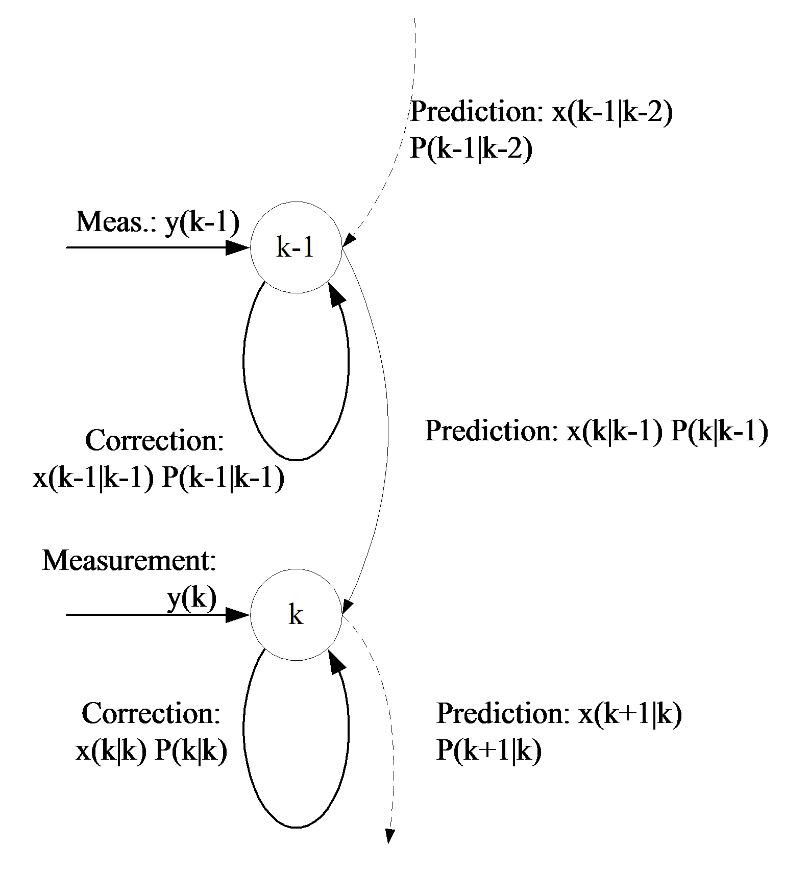
b.) Calculation of the Kalman gain:
| (.8.51) |
c.) Correction phase:
| (.8.52) |
The functionality of these equations is shown in Figure 87. The Figure 88. shows the state flow of the Kalman Filter algorithm. As a first step, the state variable x must be chosen, and the initial value of the covariance matrix P must be given. After that the algorithm will estimate the value of the state variable in each sampling period, and determine the P matrix. Let us see step by step how it works properly.
Prediction phase: In this phase, according to equation (8.50), we calculate the value of the state variable vector and the intermediate values of the covariance matrix.
Calculation of error: From the calculated and measured values (y), we will determine the error of the estimation (8.51). This value is used afterwards to calculate the Kalman gain.
Correction phase: This is the last step of the algorithms. With the help of the Kalman gain (8.52) a more accurate x value will be determined and the final value of the covariance P matrix will be evaluated, too. These steps must be effectuated for every sampling period. A flow-chart of the algorithms’ functionality is presented in Figure 88.
8.5.5. Extended Kalman Filter
In case of the induction motor the state-space model is not linear because it contains the self-product of the state variables. So the KF treated above is not applicable, we have to turn to the extension of the KF which is also suitable for nonlinear systems. The essence of the method stems from linearization of the nonlinear model, which means that we use the first derivatives of the system and we will write the filter structure according to this. In the following, for the sake of simplicity, we will notate the vectors in the kth state with  ,
,  or
or  .
.  . The nonlinear system model in this case is
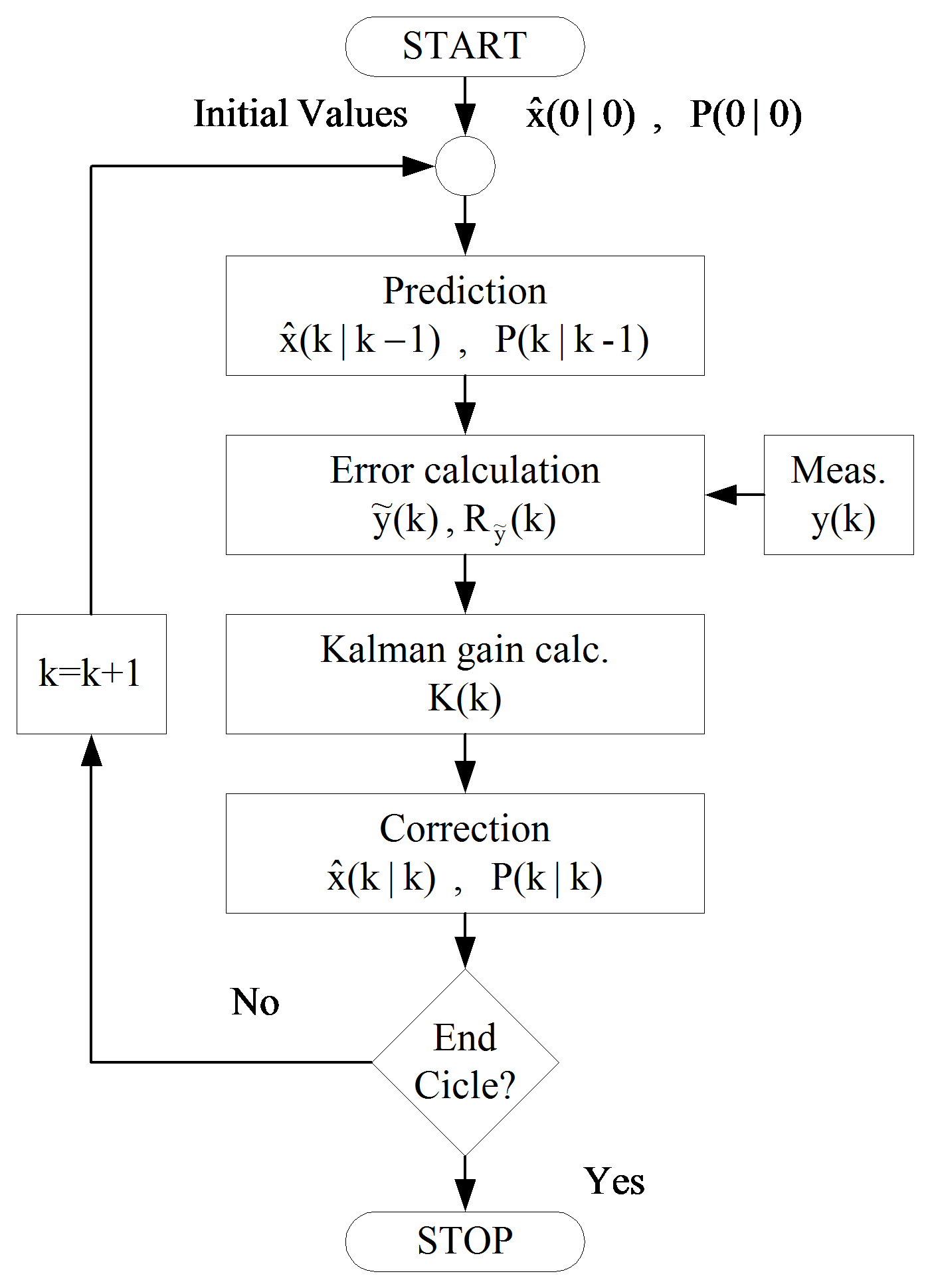
| (,8.53) |
were  and
and  are nonlinear functions of
  . The
. The  and
and  functions will be approximated by Taylor series, and in this case we obtain a linear equation. The accuracy of the approximation depends on the grade of the Taylor series.
| (,8.54) |
where the elements of matrices and
and  are the partial derivatives of
  and
and  according to
  :
:
| (.8.55) |
We will use first order Taylor series, so we can neglect the higher order terms (HOTs), and, with the help of Taylor series, we can give the model in a linearized form:
| (,8.56) |
where  .
.
Because the form of these equations is similar to that in the linear case, we can write the EKF equations according to equations (8.50), (8.51), and (8.52).
a.) Prediction phase:
| (.8.57) |
b.) Kalman gain calculation:
| (.8.58) |
c.) Correction phase:
| (.8.59) |
Of course, in this case  and
and  are the covariances of the w and v noises. If we compare the equations, we can conclude that the only difference is in the A and C matrices.
8.6. Applicability of the Kalman Filter
The Kalman filter provides a solution that directly cares for the effects of the disturbance noises. The errors in the parameters will normally be handled as noise, too. Let us recall again the state-space model of the system with the following equations, and with practically accepted notations:
| (,8.60) |
| (,8.61) |
where r and are the system noise and the measurement noise. Now we assume that these noises are stationary, white, uncorrelated and Gauss noises, and their expected values are 0. Let us now define the covariance matrices of these noises:
| (,8.62) |
| (,8.63) |
where E{.} denotes the expected value. The overall structure of the Kalman filter is the same as that of the Luenberger observer in , the only difference being in the Kalman filter matrix K as it is shown in Figure 8-9. The system equations are also the same:
| (.8.64) |
Let us introduce the reconstruction error  :
:
| (.8.65) |
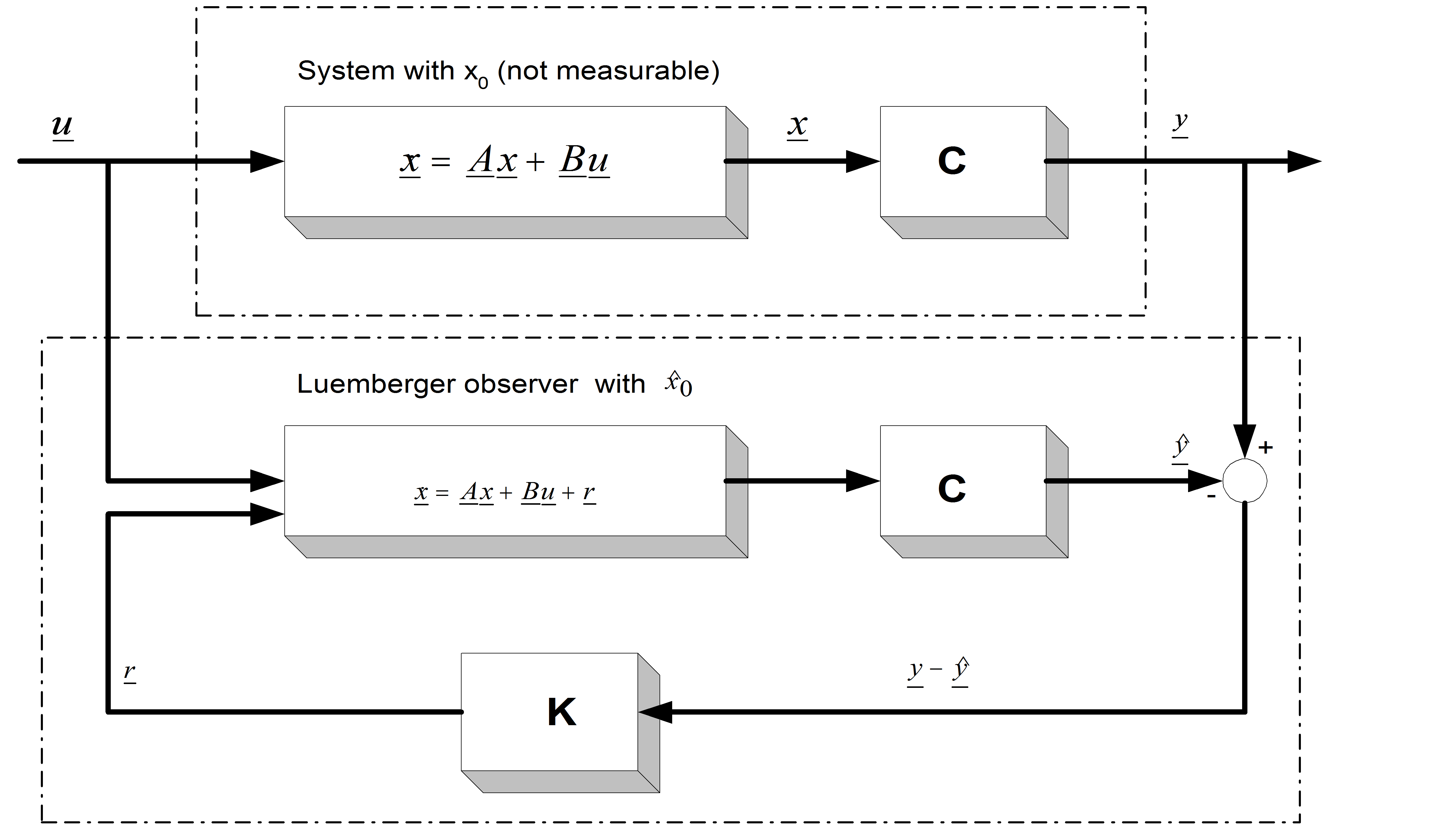
Following the substitutions as described earlier, we get:
| (.8.66) |
Hence, if K is chosen so that the system in (8.66) is asymptotically stable, the reconstruction error will always converge to zero. If the model structure is given (e.g. a deterministic state space model described in previous chapter but the matrices A, B, and C depend on such parameters that can only be measured inaccurately or cannot be measured at all, these model parameters have to be estimated from the measurements of the input and the output values. A loss function is employed to measure the output error r shown in Figure 8-9. In the case of asynchronous motors, the state space model in fact is dependent e.g. on the rotor resistance Rr, which cannot be measured accurately and changes slowly as the temperature of the motor varies. The estimation of this parameter is very important because its accuracy greatly influences the performance of the control algorithm. We will follow the notations of [24], and denote the matrix of the Kalman filter by K. The only real difference between the Luenberger observer and the Kalman filter is in the setting of the K matrix. Doing this will be based on the covariance of the noises. We will first build the measure of the goodness of the observation, which is the following:
| (.8.67) |

This depends on the choice of K. K has to be chosen to make J minimal. The solution of this is the following (see [23]):
| (,8.68) |

where P can be calculated from the solution of the following equation (Ricatti):
| (.8.69) |
Q and R have to be set up based on the stochastic properties of the corresponding noises. Since these are usually unknown, they are used as weight matrices in most cases. They are often set equal to the unit matrix, avoiding the need of deeper knowledge of the noises. In [24] a recursive algorithm is presented for the discrete time case to provide the solution for this equation. This algorithm is in fact the EKF (Extended Kalman Filter) algorithm, because the matrix of the Kalman filter, K, will be calculated on-line. The EKF is also capable of handling non-linear systems, such as the induction motor. In this case we do not have the optimum behaviour, which means the minimum variance, and it is also impossible to prove the convergence of the model. (See [25] and [23]). Let us now see the recursive form of the EKF as given in [19]. (This is basically the same as in , but with slightly different notations). All symbols in the following formulas denote matrices or vectors. They are not denoted with special notations because there is no possibility of mixing them up with scalars:
| (,8.70) |

, (8.71)
| (,8.72) |
| (,8.73) |
| (,8.74) |
where
| (,8.75) |

| (.8.76) |
These are the system vector and the output vector, respectively, and they can be explicitly calculated. The matrix K is the feedback matrix of the EKF. This matrix determines how the state vector of the EKF is modified after the output of the model is compared with the real output of the system. At this point it is important to mention that this system of equations contains many matrix operations, which can be difficult to implement in real-time. To implement this recursive algorithm, we will of course need the model of the motor, which means the matrices A, B, and C, from which we have to calculate the matrices and h. So, let us see again the motor model in this new context.
8.7. Motor model considerations
The most important thing in the following steps is the adaptation of the motor model to the Kalman Filter algorithms. This means that the motor equation must be included in the Kalman Filter model. The two main tasks are the following: first the estimation of the rotor speed, then the estimation of rotor resistance. For estimating the speed, two different co-ordinate systems will be used:
Stationary two-phase co-ordinate system, fixed to the stator;
Rotating co-ordinate system, fixed to the rotor flux.
8.7.1. Estimating the rotor speed
For parameter estimation the equations of the motor model must be given in discrete form. Looking at previous chapter it can be realized that the motor model was deduced in the continuous case, so it is now necessary to give the model in the discrete case. During discretization the higher order terms are neglected because the square of the sampling time or its values at a higher power are approximately zero. So the discrete model state matrix (“A” matrix) corresponds to the sum of the continuous model A matrix multiplied by the sampling time (T) added to the unity matrix. The discrete time “B” matrix is nothing else but the continuous time „B” matrix multiplied by the sampling time (T). In the equation  is the discrete time state matrix and
  is the discrete time „B” matrix. The model of the AC motor, as it was analyzed before is based mostly on [19], [26], and [25].
| (8.77) |

In the following the „A” and „B” matrices symbolize the discrete ones, and, according to these, the motor model will have the form as follows:
| (.8.78) |
8.7.2. Estimation of speed on the stationary reference frame
Equation (8.78) is the starting or reference equation, which was used during the estimation and has been adapted to the Kalman Filter (KF). The KF is applicable to predict or estimate only the state variables of the model, so the speed of the rotor  must be included in the set of state variables. We do not give a formula for calculating the speed
  , we only use the assumption that
  , which is a good approximation during one sampling period. Therefore, in the prediction phase, the speed values are identical with the values in the previous state. In the correction phase, the rotor speed will be modified according to the measured
  values (see equation (8.53) ). Further, because
  is included in the state variable matrix, the model is not linear anymore, so we have to turn to the extended Kalman Filter. In this case, the general equation of the model has been changed slightly because of the nonlinearities:
| (.8.79) |
In the case of the motor model, there is a linear relationship between the output ( ) and the input (
 ), and this is why the C matrix is used instead of the “g” function (8.53). The state model in the nonlinear case is the following:
| (.8.80) |
Let us analyze the nonlinear „f” function:
| (8.81) |
We do not need to give the “g” function in the model because the C matrix is linear. To effectuate the estimation, we further need the partial derivatives of the function “f”. This matrix is sometimes denoted by „A”, and in this case the equations are very similar to the equations in the case of a linear filter.
| (8.82) |
In the calculation of the y we use linear equations:
| (8.83) |
These equations will go into the equations of the Kalman Filter.
8.7.3. Estimation of speed in a rotating reference frame
In this section we will estimate the rotor speed in a d-q reference frame fixed to the rotor flux. The equations are borrowed from the FOC control of induction motors, and are extended with the motion/kinetic equation of the motor. The advantage of this method is that the speed is approximated according to the motion equation, which is done in the prediction phase, and then followed by a correction, which is done with the help of the measured data. In the previous case of the α- stationary co-ordinate system we did not use the motion equation, so in the present case the filter structure is more complex than it was in the previous case. Let us see the new state variables and the model itself. The magnetizing current, which was dealt with in previous chapter in the case of FOC , has appeared as a state variable In this case the estimation is based on the following equations. The first three are the stator current equations in a d-q co-ordinate system and the fourth one is the kinetic equation:
| (,8.84) |

| (,8.85) |
| (,8.86) |
| (,8.87) |
It can be observed that the last equation contains the product of the q component of the stator current and the magnetizing current. Let us now identify again the state variables, the inputs and the outputs. The state variable is a 4th order vector, containing the stator current components, the magnetizing current, and the speed of the rotor. The output (y) of the filter is the α- stationary components of the stator current vector. The stator voltage is the input of the model.
| (8.88) |
Equation (8.87) has been deduced from the equation borrowed from the modelling of asynchronous motor, which is the basic kinetic equation of the motor. It can easily be observed that the speed of the motor depends intensively on the electromagnetic torque and the load torque. The load torque is one input of the model and can be considered as a disturbance: The electromagnetic torque expression has been presented also in previous chapter and these equations will be repeated here for convenience:
![]() is the rotor flux speed in the stationary reference frame. For the calculation of the speed we can proceed in two ways:
is the rotor flux speed in the stationary reference frame. For the calculation of the speed we can proceed in two ways:
a) ![]() ,as a constant:
,as a constant:
The essence of this method relies on the equation below, where we consider the rotor flux speed as a constant value and we calculate the slip and the rotor speed outside the KF. This approach considerably simplifies the system model:  .
.
Let us see what it looks like:
| (.8.89) |
The partial derivative matrix of „f” is the following:
| (8.90) |

b) ![]() inserted into the filter model:
inserted into the filter model:
In this case we use (8.91) equation for calculating ![]() :
:
| (,8.91) |
The equation has three state variables: the magnetizing current, the “q” component of the stator current, and the speed of the rotor. These state variables will complicate the model and the partial derivatives matrix of “f”. Another draw-back of this method is that if the magnetizing current is zero, the value of ![]() cannot be determined. This means that we have to check the value of the magnetizing current in each sampling period. Let us see now the form of the „f” function and its partial derivatives in these circumstances:
cannot be determined. This means that we have to check the value of the magnetizing current in each sampling period. Let us see now the form of the „f” function and its partial derivatives in these circumstances:
| (8.92) |
| (8.93) |
The input of the model in both cases is the stator voltage, in a stationary reference frame.
8.7.4. Estimating the rotor resistance
Until now the value of the rotor resistance has been considered as a constant, and the model of the motor has been deduced according to this assumption. It is well known that during motor operation this value can change considerably, and this depends to a great extent on the internal temperature of the motor. To give an analytical equation to these considerations is very difficult, so we will consider these factors as noise in the system. Mostly in the range of low speed operation (where the temperature of the motor increases), the value of the rotor resistance does not absolutely match with its constant value. In this case we use a KF filter to approximate the value of the rotor resistance and to increase the accuracy of the model. Let us see now how this is implemented. The rotor flux speed is not introduced in the filter model. The estimation of Rr can be effectuated also for the second case b) above, the steps are the same. Now we have to include Rr in the state variable matrix as shown below:
| (.8.94) |
The output and the input of the system are kept as before. The rotor time constant has been extracted from the formula of the function “f” because this term depends on the rotor resistance:
| (.8.95) |

Inserting the „f” function into equation (8.92) we will have the following formula:
| (.8.96) |
As it can be seen, we do not give any formulae for calculating Rr, which, from the point of view of the filter, means that we do not have a prediction phase. Therefore, the value of Rr is identical with its previous value in the prediction phase (8.57). The approximation of Rr is made by the KF in the correction phase. The matrix of partial derivatives of the function „f” will be
| (.8.97) |
These formulae will be inserted into the model of the filter. This will be the last step to enable both real-time implementation and simulation. Let me now summarize the main design steps for a speed-sensorless induction motor drive implementation using the discretized EKF algorithm.
The steps which sould be made are as follows:
Selection of the time-domain induction machine model;
Discretization of the induction machine model;
Determination of the noise and state covariance matrices , R, P;
Implementation of the discretized EKF algorithm; tuning.
The above design steps will be shortly discussed:
1. For the purpose of using an EKF for the estimation of the rotor speed of an induction machine, it is possible to use various machine models. For example, it is possible to use the equations express in the rotor-flux-oriented reference frame, or in the stator-flux-oriented reference frame. When the model expressed in the rotor-flux-oriented reference frame is used, the stator current components in the rotor-flux-oriented reference frame are also state variables and the input and output matrices contain the sine and cosine the angle of the rotor flux-linkage space vector. These transformations introduce extra non-linearities, but these transformations are not present in the model established in the stationary reference frame. The main advantages of using the model in the stationary reference frame are:
Reduced computation time (e.g. due to reduced non-linearities);
Smaller sampling times;
Higher accuracy;
More stable behavior.
2. The discretization of the model has been treated extensively previously so in this place we omit the treatment again.
3. The goal of the Kalman filter is to obtain unmeasurable states (rotor speed) by using measured states, and also statistics of the noise and measurements (covariance matrices Q,R,P of the system noise vector, measurement noise vector, and system state vector respectively). In general, by means of the noise inputs, it is possible to take account of computational inaccuracies, modelling errors, and errors in the measurements. The filter estimation is obtained from the predicted values of the states and this is corrected recursively by using a correction term, which is the product of the Kalman gain and the deviation of the estimated measurement output vector and the actual output vector.The Kalman gain is chosen to result in the best possible estimated states. Thus the filter algorithm contains basically two main stages, a prediction stage and a filtering stage. During the prediction stage, the next predicted values of the states are obtained by using a mathematical model (state-variable equations) and also the previous values of the estimated states. Furthermore, the predicted state covariance matrix (P) is also obtained before the new measurements are made, and for this purpose the mathematical model and also the covariance matrix of the system (Q) are used. In the second stage, which is the filtering stage, the next estimated states, are obtained from the predicted estimates by adding a correction term  to the predicted value. This correction term is a weighted difference between the actual output vector and the predicted output vector where K is the Kalman gain.
Thus the predicted state estimate (and also its covariance matrix) is corrected through a feedback correction scheme that makes use of the actual measured quantities. The Kalman gain is chosen to minimize the estimation-error variances of the states to be estimated. The computations are realized by using recursive relations. The algorithm is computationally intensive, and the accuracy also depends on the model parameters used. A critical part of the design is to use correct initial values for the various covariance matrixes.
These can be obtained by considering the stochastic properties of the corresponding noises. Since these are usually not known, in most cases they are used as weight matrices, but it should be noted that sometimes simple qualitative rules can be set up for obtaining the covariances in the noise vectors. The system noise matrix Q depending on the model is a five-by-five matrix, the measurement noise matrix R is a two-by-two matrix, so in general this would require the knowledge of 29 elements. However, by assuming that the noise signals are not correlated, both Q and R are diagonal, and only 5 elements must be known in Q and 2 elements in R. However, the perameters in the direct and quadrature axes are the same, which means the two first elements in the diagonal of Q (q11=q22) are equal, the third and fourth elements in the diagonal of Q (q33=q44) are equal so Q=diag(q11,q11,q33,q33,q55) contains only 3 elements which have to be known. Similarly, the two diagonal elements in R (r11=r22) are equal, thus R=diag(r11,r11). It follows that in total only 4 noise covariance elements must be known.
As discussed above, the EKF is an optimal, recursive state estimator, and the EKF algorithm contains basically two main stages, a prediction stage and a filtering stage. The EKF equation is:
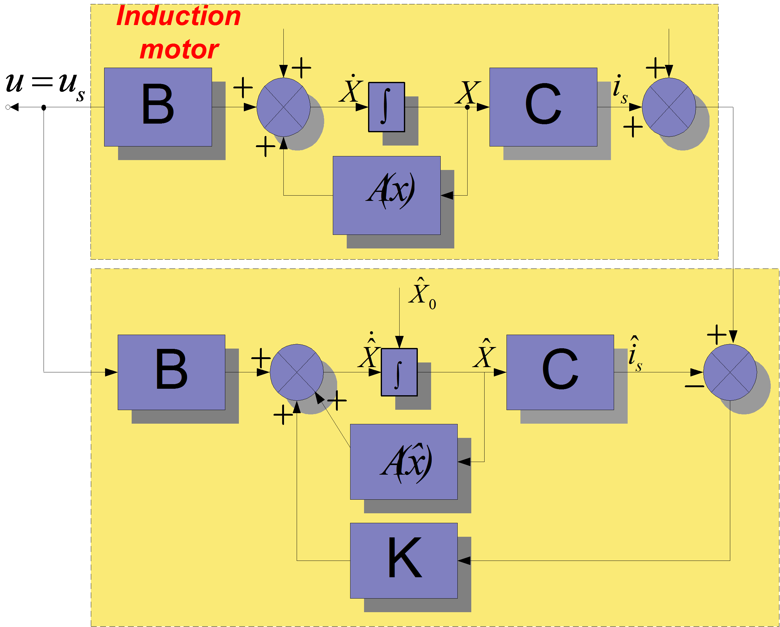
| (8.98) |
The structure of the EKF is shown in Figure 8-10.
The starting-state covariance matrix can be considered as a diagonal matrix, where all the elements are equal. The initial values of the covariance matrices reflect on the degree of knowledge of the initial state: the higher their values, the less accurate is any available information and the convergence speed of the estimation process will increase. However, divergence problems, or large oscillation of state estimates around a true value may occur when too high initial covariance values are chosen. A suitable selection allows us to be obtain satisfactory speed convergence, and avoids divergence problems or unwanted large oscillations.
The accuracy of the state estimation is affected by the ammont of information that the stochastic filter can extract from its mathematical model and the measurement data processing. Some of the estimated variables, especially unmeasured ones, may indirectly and weakly be linked to the measurement data, so only poor information is available to the EKF. Finally it should be noted that another important factor which influences the estimation accuracy is due to the different size of the state variables, since the minimization of the errors for the variables with small size. This problem can be overcome by choosing normalized state-variables. For the realization of the EKF algorithm it is very convenient to use a signal processor (e.g. Texas Instruments TMS320C30, TmS320C40, TMS320C50, etc.), due to the large number of multiplications required and also due to fact that all of the computations have to be performed fast: within one sampling interval. The calculation time of the EKF is 130  s on the TMS320C40. However, the calculation times can be reduced by using optimized machine models.
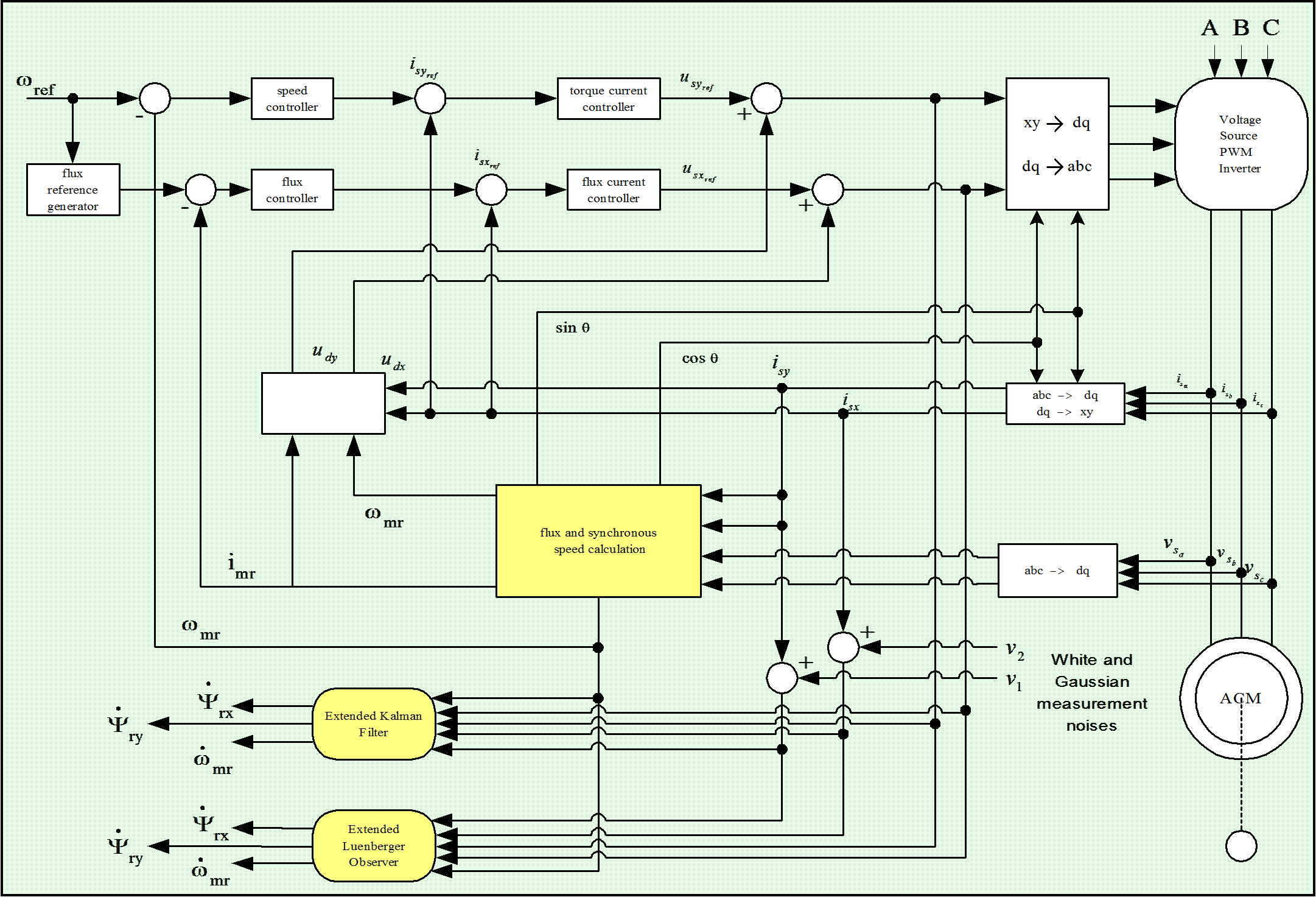
The EKF described above can be used under both steady-state and transient conditions of the induction machine for the estimation of the rotor speed. By using the EKF in the drive system, it is possible to implement a PWM inverter-fed induction motor drive without the need of an extra speed sensor. It should be noted that accurate speed sensing is obtained in a very wide speed-range, down to very low values of speed (but not zero speed). However, care must be taken in the selection of the machine parameters and covariance values used. The speed estimation scheme requires the monitored stator voltages and stator currents. Instead of using the monitored stator line voltages, the stator voltages can also be reconstructed by using the d.c. link voltage and inverter switching states, but especially at low speeds it is necessary to have an appropriate dead-time compensation, and also the voltage drops across the inverter Switches (e.g. MOSFETs, IGBTs) must be considered. Furthermore in a VSI inverter-fed vector-controlled induction motor drive, where a space-vector modulator is used, it is also possible to use the reference voltages (which are the inputs to the modulator) instead of the actual voltages, but this requires appropriate error compensation.
The tuning of the EKF involves an iterative modification of the machine parameters and covariance in order to yield the best estimates of the states. Changing the covariance matrices Q and R affects both the transient duration and steady-state operation of the filter. Increasing Q corresponds to stronger system noises, or larger uncertainty in the machine model used. The filter gain matrix elements will also increase and thus the measurements will be more heavily weighted and the filter transient performance will be faster. If the covariance R is increased, this corresponds to the fact that the measurements of the currents are subjected to a stronger noise, and should be weight less by the filter. Thus the filter gain matrix elements will decrease and this results in slower transient performance. Finally it should be noted that in general, the following qualitative tuning rules can be obtained: Rule 1: If R is large then K is small (and the transient performance is faster). Rule 2: If Q is large then K is large (and the transient performance is slower). However, if Q is too large or if R is too small, instability can arise. In summary it can be stated that the EKF algorithm is computationally very intensive, but it can also be used for joint state and parameter estimation. It should be noted that to reduce the computational effort and any steady state error, it is possible to use various EKFs, which utilize reduced-order machine models and different reference frames (e. g. a reference frame fixed to the stator current vector).
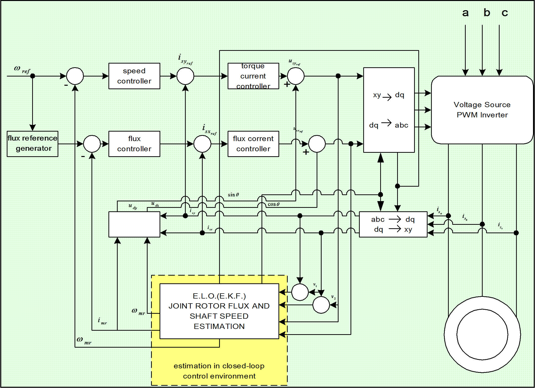
8.8. Realization of the Kalman Filter
Reaching this point, the realization of the model in Matlab/Simulink can begin. The strategy for implementing the Kalman Filter based method was the following: before introducing the filter on the feed-back line, first we used off-line identification methods as shown in Figure 8-11. [25]. As it can be seen on the figure, a traditional FOC method was used for testing the performance of the estimation. When the estimated values match the values of the system, the observers can be inserted in the feedback loop for achieving the on-line identification of the desired parameters. In the closed loop environment both the rotor flux and the rotor’s angular speed are also estimated, so we do not need any flux model or flux calculation procedure. The realized model structure can be seen in Figure 8-12. Realizing the complete Kalman filter as a Simulink model would have resulted in a very complicated model, and it seemed easier to implement it simply as a Matlab language file. Another advantage of this is that the Matlab language file can more easily be converted into an assembly program. A subsystem was inserted into the system that contains the Kalman filter, which is then built into the model as an S-function. The overall structure of the controller has not been changed very much. The filter is in the subsystem called KF. Its output depends on which model we use. The Figure 8-13. shows the case of the EKF with the second motor model from [19]. In this case, the outputs of the system are all state variables: the rotor fluxes, the stator currents, and the rotor speed. The inputs are measured rotor currents and rotor voltages. In the other case, the output would be only the rotor speed, but the estimated rotor speed would be needed as well, which sould be calculated by a flux model.
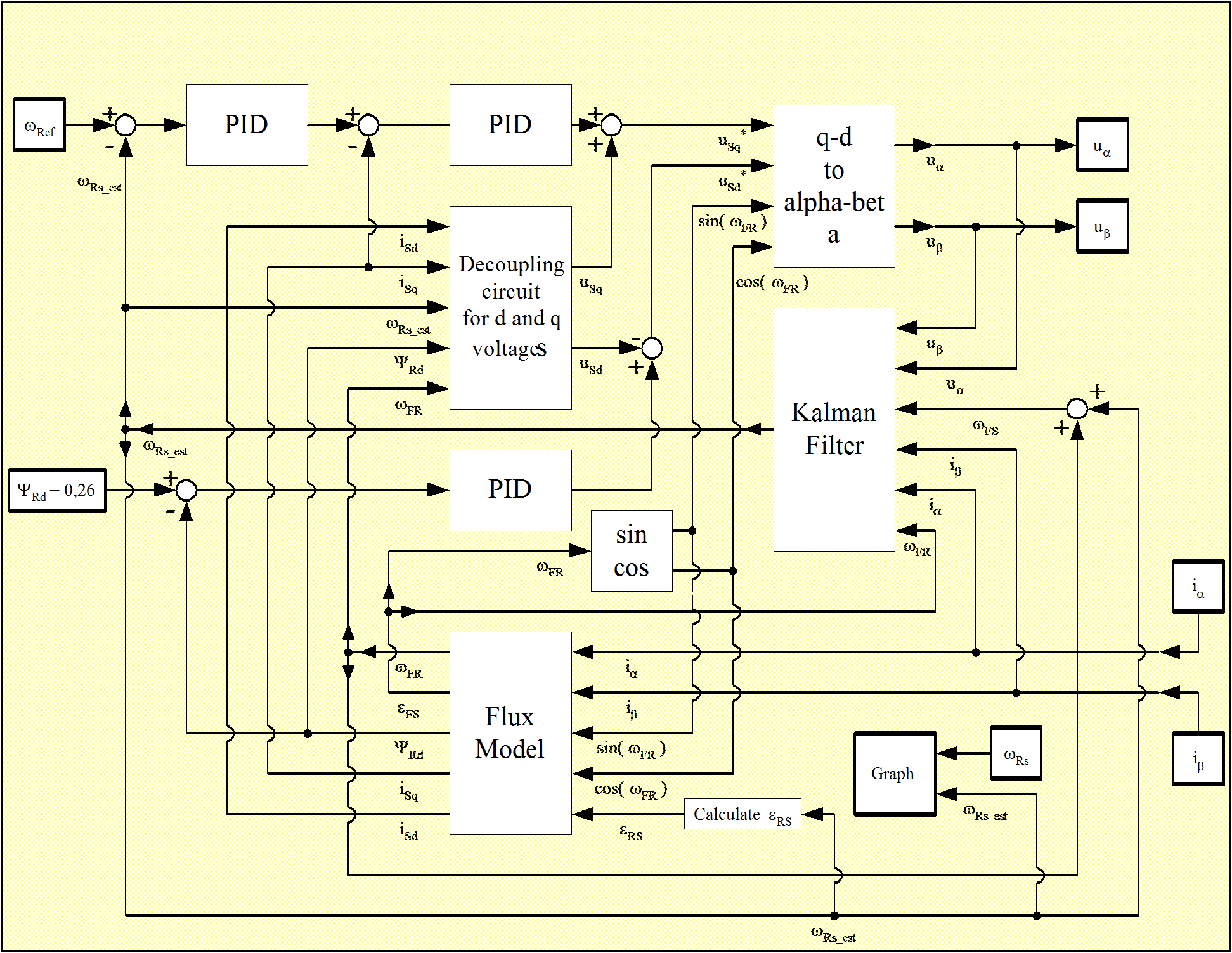
These tests reveal that the model of Vas presented in [26] has a much more stable behavior. After achieving the required simulation results, real-time implementation could begin, based again on the second model.
Chapter 9. Glossary of SYMBOLS

magnetical axis of phase a in the stator
aphase a in a three-phase system
arotational unit vector of 120°

rotational unit vector of 240°
[A]phase transformation matrix
bphase b in a three-phase system
cphase c n a three-phase system
Ccondenser capacity
Dfixed of stator-oriented direct axis
Ddiode
[D]rotational matrix operator of a two-phase axis system

arbitrarily rotating of field-oriented direct axis

air-gap field-oriented direct axis

resultant rotor field-oriented direct axis

resultant stator field-oriented direct axis

rotor-oriented direct axis

space phasor of the electromotive force

stator voltage and stator current frequency

stator current oriented direct axis

space vector or space phasor of a current

armature current in a DC machine

active component of the current space phasor

 DC link current

magnetizing current

rotor-flux based magnetizing current

stator-flux based magnetizing current
Rereal axis of the complex plane and real part of the complex expression
Imimaginary axis of the complex plane and imaginary part of the complex expression

rotor current

reactive component of the current space phasor

stator current
jrotational unit vector of 90°
[j]rotational matrix operator of 90° for a two-phase system of magnitudes without zero-sequence component
Jtotal equivalent moment of inertia

proportional coefficient between the magnitude of the stator current space phasor and the d.c. link current
Ktorque constant of a DC machine
[K]rotational matrix operator of 90° for a three-phase system of magnitudes

space phasor definition (constant) coefficient

referring constant of the currents and magneto motoric force

torque constant of an AC machine

torque constant of the induction machine containing the rotor leakage coefficient

torque constant of the induction machine containing the stator leakage coefficient

power coefficient matrix

referring constant of the resistances and inductances

scale coefficient of the space phasor

reffering constant of the voltages and electro motoric force

inductance of the main magnetic circuit

useful inductance of the rotor-phase winding

total per-phase inductance of the rotor

useful inductance of the stator-phase winding

total per-phase inductance of the stator

rotor’s own per-phase leakage inductance

stator’s own per-phase leakage inductance

inductance of the thyristor commutation coil

DC link current filtering inductance

three-phase resultant mutual (useful) inductance

three-phase resultant (total) rotor inductance

zero-sequence inductance of the rotor

three-phase resultant (total) stator inductance

zero-sequence inductance of the stator

resultant leakage inductance of the rotor

resultant leakage inductance of the stator
mmutual inductance between a stator and a rotor phase

electromagnetic torque

dynamic torque

resistent load torque

mutual leakage inductance between two rotor phases

mutual leakage inductance between two stator phases

number of rotor phases

number of stator phases
[q]matrix of the oscillator output quantities
pinstantaneous power or power losses

instantaneous mechanical power

projection of a space vector or space phasor
qfixed or stator-oriented quadrature axis
[Q]rotational matrix of 90° for a two-phase system of magnitudes including the zero-sequence component

stator-current oriented quadrature axis

arbitrarily rotating or field-oriented quadrature axis

air-gap field-oriented quadrature axis

resultant rotor field-oriented quadrature axis

resultant stator field-oriented quadrature axis

rotor-oriented quadrature axis
Rereal axis of the complex plane
Rereal part of a complex expression

resistance of diode

rotor per-phase resistance

stator per-phase resistance

resistance of thyristor or transistor
ttime
[t]three-phase projection matrix
[T]rotational matrix operator of three-phase axis system

space phasor of voltage

voltage drop

DC link output/inverter input voltage

rotor voltage

rectifier output/DC link input voltage

stator voltage
Nturn number of winding

number of the poli-pairs

angular position of the magnetizing-current space phasor

angular position of the rotor-current space phasor

angular position of the stator-current space phasor

angular position of an arbitrarily rotating direct axis or of a field-oriented axis

angular position of the air-gap resultant flux space phasor

angular position of the rotor resultant flux space phasor

angular position of the stator resultant flux space phasor

electrical angular position of the rotor  axis
axis

mechanical angular position of the rotor  axis
axis

resultant (total) leakage coefficient

rotor leakage coefficient

stator leakage coefficient

space vector or space phasor of flux linkage

space vector of armature reaction flux in DC machine

space vector of compensating flux in DC machine

space vector of exciting flux

air-gap flux

resultant rotor flux

resultant stator flux

rotor leakage flux

rotational matrix of three-phase axis system, when the zero-sequence component is missing

time constant of the rotor

time constant of the stator

electrical angular speed of the rotor

synchronous electrical angular speed

mechanical angular speed of the rotor

rotational speed of the magnetizing-current space phasor

rotational speed of the rotor-current space phasor

rotational speed of the stator-current space phasor

angular speed of an arbitrarity rotating axis system or of a field-oriented axis

rotational speed of the air-gap flux space phasor

rotational speed of the resultant rotor flux space phasor

rotational speed of the resultant stator flux space phasor
NAME | Symbols within the text | Symbols within the formulae describing implementations and simulations |
Stator and rotor currents |
| iS, iR |
Stator current three-phase co-ordinates |
| iS_a, iS_b, iS_c |
two-phase co-ordinates |
| iS_alpha, iS_beta |
field co-ordinates |
| iS_d, iS_q |
Magnetising current |
| ImR |
Stator voltage |
| US |
Rotor flux |
| Psi_R |
Rotor, rotor flux and slip angular velocity |
| omega_Rotor, omega_Flux, omega_Slip |
Reference speed |
| Omega_ref |
Rotor, rotor flux and slip angle |
| eps_Rotor,eps _Flux eps_Slip |
Load torque |
| torque_L |
Stator and rotor resistance and Time constants |
| Rs, Rr, Ts, Tr, |
Stator, rotor and main inductance |
| Ls, Lr, Lm |
Leakage factor |
| Sigma |
Number of poles |
| P |
Moment of inertia |
| J |
System noise variance |
| - |
Output/Measurement noise variance |
| - |
Kalman gain | K | K |
Estimated motor state variable |
| i_alpha_est; i_beta_est Psi_R_alpha_est; Psi_R_beta_est i_d_est; i_q_est - |


9.1. Mathematical Symbols
cross vectorial product
complex conjugate
element of (contained in)
not element of (not contained in )
null set
implication
biimplication
negation (complement)
identity
equivalence
union (disjunction)
OR
intersection (conjunction)
AND
ordered pair
Cartesian product
fuzzy intersection operator (fuzzy AND), T-norm
fuzzy union operator (fuzzy OR), S-norm, T-conorm
subset of (A’ÍB’ means that A’ is subset of B’)
proper subset of (A’ÌB’ means that A’ is proper subset of B’)
not proper subset of
Ttranspose
Xuniverse of discourse (sample space)
ççx - yúú Euclidean distance between vectors x and y
mmembership function, MF (degree of belongingness)
x1, x2, …symbol 125 \f "Symbol" \s 10crisp set of numbers
9.2. General abbreviations
AI artificial intelligence
AIB artificial-intelligence-based
ANN artificial neural network
ASM asynchronous motor
CSI current source inverter
DSP digital signal processor
DTC direct torque control
EKF extended Kalman Filter
ELO extended Luenberger Observer
FLC fuzzy logic controller
FLEOC fuzzy logic efficiency optimizer controller
FLSfuzzy logic system
GA genetic algorithm
IM induction machine
KFKalman Filter
LO Luenberger Observer
MRAC model reference adaptive control
NRAS model reference adaptive system
NARMAX non-linear auto regressive moving average model
p.m. permanent magnet
PWM pulse-width modulator/modulation
SRM switched reluctance machine
SYRM synchronous reluctance machine
TDL tapped delay line
VSI voltage source inverter
9.3. Abbreviations for fuzzy sets
NL negative large
NM negative medium
NS negative small
ZE zero
PS positive small
PM positive medium
PL positive large
References
[1] Variable Structure Control Optimization. 1992. Springer-Verlag.
[2] Controller Design for Manipulator using Theory of Variable Structure Systems. 101-109. 1978. IEEE Trans. on System, Man, and Cybernetics.
[3] 1st IFAC Congress. . Application of the theory of differential equations with discontinuous right-hand sides to non-linear problems in autimatic control. 923-925. 1960.
[4] Differential equations with discontinuous right-hand side. 199-231. 1964. Ann. Math Soc. Transl..
[5] Sliding Mode Design for Motion Control. 2000.
[6] 2nd Eur. Conf. On Power Electronics, Proc., pp 251-256. Grenoble. . Sliding Mode Control for Robotic Manipulators". 1987.
[7] Microprocessor Based Robot Manipulator Control with Sliding Mode". 1. 11-18. 1987. IEEE Trans. On Industrial Electronics.
[8] Application of Sliding Modes to Induction Motor. 1. 4149. 1981. IEEE Trans. On Industrial Appl..
[9] EDIS – Publishing Centre of Zilina University, ISBN 80-8070-087-7. Zilina. Forced Dynamics Control of Electric Drive. 2003.
[10] Methods for constructing discountnuous planes in multidimensional variable structure systems. 10. 1466-1470. Oct. 1978. Automat. Remote Control.
[11] Sliding-mode control for high precision motion of a piezostage. 1. 629-637. Feb. 2007. IEEE Trans. Ind. Electron..
[12] Robust fuzzy neural network slidingmode control for two-axis motion control system. 4. 1209-1225. June 2006. IEEE Trans. Ind. Electron..
[13] Network-based fuzzy decentralized sliding-mode control for cat-like mobile robots. 1. 574-585. Feb. 2007. IEEE Trans. Ind. Electron..
[14] Berlin. Technische Universität Berlin. Vergleichende Untersuchungen von unterschiedlichen feldorienten Lagerstrukturen für Asynchron-Servomotoren mit einem Multi-Transputer-System, Dissertation. 1992.
[15] Texas Instruments. Sensorless Field Oriented Control with Kalman Filter for Asynchronous Drives Using a Fixed-Point Signal Processor. 1996.
[16] Springer-Verlag. Control of Electrical Drives. 1985. Springer-Verlag.
[17] Oxford Science Publications. Sensorless Vector Control and Direct Torque Control. 1998.
[18] OMIKK. Budapest. Vector Control of AC Drives. 1991.
[19] Einsatz eines Kalman-Filters zum feldorientierten Betrieb einer Asynchronmaschine ohne mechanische Sensoren. 1990.
[20] IEEE Industrial Electronics Society. . Sensorless Control of AC Motor Drives. 1997. IEEE Industrial Electronics Society.
[21] Conf. Rec. IEEE-IECON’94. . Comparison of Different Schemes without Shaft Sensors for Field Oriented Control Drives. 1579-1588.
[22] Prentice-Hall. Computer-Controlled Systems. 1990.
[23] A Comparative Study of Rotor Flux Estimation in Induction Motors with Nonlinear Observer and the Extended Kalman Filter.
[24] R. Oldenbourg Verlag. München-Wien. Kalman-Bucy Filter, Deterministische Beobachtung und stochastische Filterung. 1994.
[25] Design and application of extended observers for joint state and parameter estimation in high-performance AC Drives. No.2. 1995. IEE Proc.-Electr.Power Appl..
[26] Intelligent Motion Proceedings. Application of Kalman Filters and Extended Luenberger Observers to Induction Motor Drives. 1994.
[27] A microprocessor-controlled speed regulator with instantaneous speed estimation for motor drives. 1. 95-99. Feb. 1988. IEEE Trans. Ind. Electron..
[28] Control Engineering. Red Business Information. Loop Tuning Fundamentals. July 1, 2003.
[29] Application of fully decoupled parity equation in fault detection and identification of dcmotors. 4. 1277-1284. June 2006. IEEE Trans. Ind. Electron..
[30] Determination of scaling factors for fuzzy logic control using the sliding-mode approach: Application to control of a dc machine drive. 1. 296-309. Feb. 2007. IEEE Trans. Ind. Electron..
[31] Energy-management system for a hybrid electric vehicle, using ultracapacitors and neural networks. 2. 614-623. Apr. 2006. IEEE Trans. Ind. Electron..
[32] Fuzzy controllers with maximum sensitivity for servosystems. 3. 1298-1310. Apr. 2007. IEEE Trans. Ind. Electron..
[33] A high-performance sensorless indirect stator flux orientation control of industion motor drive. 1. 614-623. Feb. 2006. IEEE Trans. Ind. Electron..
[34] On Carath_Eodory's Conditions For The Initial Value Problem. 5. 1371{1376 S 0002-9939(97)03942-7 . 1997. Proceedings Of The American Mathematical Society.
[35] 1st IFAC Congr., pp. 923-925. Moscow. . Application of the Theory of Differential Equations with Discontinuous Right-hand Sides to Non-linear Problems in Automatic Control. 1960.
[36] Differential Equations with Discontinuous Right-hand Side. 199-231. 1964. Ann. Math Soc. Transl..
[37] EPE'91 4th European Conference on PowerElectronics, Proceedings vol. 3. pp. 3-180-184. Firenze. . Control of a Three Phase UPS Inverter with Unballanced and Nonlinear Load. 1991.
[38] Springer-Verlag. . Park Vector Based Sliding Mode Control K.D.Young, Ü. Özgüner (editors) Variable Structure System, Robust and Nonlinear Control.ISBN: 1-85233-197-6. 6. 1999. Springer-Verlag.
[39] Invariant Sliding Sector for Variable Structure Control. 2. 124-134. 2005. Asian Journal of Control.
[40] 8th Conference on Power Electronics and Motion Control Vol. 5, pp.5-254-5-259. . . Sector Sliding Mode Controller for Motion Control. 1998.
[41] Design of variable structure controllers with continuous switching control. 3. 409-431. 1996. INTERNATIONAL JOURNAL OF CONTROL.
[42] A Singular Perturbation Analysis of High-Gain Feedback Systems. 6. 931-938. 1977. IEEE Trans. on Automatic Control.
[43] Sliding Mode Control of a Discretee System. 145-152. 1990. System Control Letters.
[44] Sliding Mode in Dynamics Systems. 1029-1037. 1992. International Journal of Control.
[45] R. Oldenbourg Verlag. München-Wien. Kalman-Bucy Filter, Deterministische Beobachtung und stochastische Filterung. 1994.
[46] Tankönyvkiadó. Budapest. Automatizált villamos hajtások I.. 1989.