Chapter 6. Sample measurement
- 6.1. Using the PCI-1720 D/A card -- Exercise 1
- 6.2. Using the real-time clock with PCI 1720 D/A card – Exercise 2
- 6.3. Using the PCI-1784 Counter card -- Exercise 3
- 6.4. Open Loop Control measurement – Motion control/Exercise 4. Open-loop test
- 6.5. Closed Loop Control Measurements -- Exercise 5
-
- 6.5.1. Parameter tuning of the P controller -- Test 1.
- 6.5.2. Step signal response of the P controller -- Test 2.
- 6.5.3. Response of the P controller to step changes in the reference speed signal -- Test 3.
- 6.5.4. Response of the P controller to step changes in the load -- Test 4.
- 6.5.5. Step signal response of the PI controller -- Test 2.
- 6.5.6. Response of the PI controller to step changes in the reference speed signal -- Test 3.
- 6.5.7. Response of the PI controller to step changes in the load -- Test 4.
- 6.5.8. Step signal response of the P and PI controller -- Test 1.
- 6.5.9. Stick-slip phenomenon
- 6.5.10. Step signal response of the position controller with inner shaft speed controller -- Test 1.
- 6.5.11. Fault tolerance measurements
- 6.5.12. Control of time-delay system
- 6.5.13. Sliding mode control results
- 6.6. Complex design and measurement
-
- 6.6.1. State feedback and its design
- 6.6.2. Application of reference signal correction
- 6.6.3. Design of the state observer
- 6.6.4. Integral control
- 6.6.5. Identification of the system
- 6.6.6. Design of the control
- 6.6.7. Identification of the motor
- 6.6.8. Design of the control
- 6.6.9. Integral control
- 6.6.10. Filter design for velocity measurement
- 6.6.11. Implementation
- 6.6.12. Control without integrator
- 6.6.13. Results of the measurement
- 6.6.14. Control with the integrator
- 6.6.15. Results of the measurement in the case of integrator
- 6.6.16. Appendix
6.1. Using the PCI-1720 D/A card -- Exercise 1
The code that is the solution and should be pasted into the code box is:
motorDA = 3;
new_voltage = 5.0;
//Step 1: Open device
dwErrCde = DRV_DeviceOpen(lDevNumDA, &lDriverHandleDA);
if (dwErrCde != SUCCESS)
{
    ErrorHandler(dwErrCde);
    exit(1);
}
// Step 2: Output value to the specified channel
tAOVoltageOut.chan = motorDA;
tAOVoltageOut.OutputValue = new_voltage;
dwErrCde = DRV_AOVoltageOut(lDriverHandleDA, &tAOVoltageOut);
if (dwErrCde != SUCCESS)
{
    ErrorStop(&lDriverHandleDA, dwErrCde);
    return;
}
This code turns on the drive unit power. You should see the green LED on the drive unit lit.
To turn off the LED modify the following line: new_voltage = 0.0;
6.1.1. From the sample file (Dasoft.cpp) the following part should be copied to the text box:
//Step 3: Open device
dwErrCde = DRV_DeviceOpen(lDevNum, &lDriverHandle);
if (dwErrCde != SUCCESS)
{
    ErrorHandler(dwErrCde);
    printf("Program terminated!\n");
    printf("Press any key to exit....");
    getch();
    exit(1);
}
// Step 4: Output value to the specified channel
tAOVoltageOut.chan = usChan;
tAOVoltageOut.OutputValue = fOutValue;
dwErrCde = DRV_AOVoltageOut(lDriverHandle, &tAOVoltageOut);
if (dwErrCde != SUCCESS)
{
    ErrorStop(&lDriverHandle, dwErrCde);
    printf("Press any key to exit....");
    getch();
    return;
}
6.1.2. Remove the code parts marked with red.
//Step 3: Open device
dwErrCde = DRV_DeviceOpen(lDevNum, &lDriverHandle);
if (dwErrCde != SUCCESS)
{
    ErrorHandler(dwErrCde);
printf("Program terminated!\n");
    printf("Press any key to exit....");
    getch();
    exit(1);
}
// Step 4: Output value to the specified channel
tAOVoltageOut.chan = usChan;
tAOVoltageOut.OutputValue = fOutValue;
dwErrCde = DRV_AOVoltageOut(lDriverHandle, &tAOVoltageOut);
if (dwErrCde != SUCCESS)
{
    ErrorStop(&lDriverHandle, dwErrCde);
printf("Press any key to exit....");
    getch();
    return;
}
6.1.3. Change the code as it is highlighted with green.
motorDA = 3;
new_voltage = 5.0;
//Step 1: Open device
dwErrCde = DRV_DeviceOpen(lDevNumDA, &lDriverHandleDA);
if (dwErrCde != SUCCESS)
{
    ErrorHandler(dwErrCde);
    exit(1);
}
// Step 2: Output value to the specified channel
tAOVoltageOut.chan = motorDA;
tAOVoltageOut.OutputValue = new_voltage;
dwErrCde = DRV_AOVoltageOut(lDriverHandleDA, &tAOVoltageOut);
if (dwErrCde != SUCCESS)
{
    ErrorStop(&lDriverHandleDA, dwErrCde);
    return;
}
Alternative solution can be achieved without using the predefined variables (motorDA and new_votlage). In this case the code is the following:
//Step 1: Open device
dwErrCde = DRV_DeviceOpen(lDevNumDA, &lDriverHandleDA);
if (dwErrCde != SUCCESS)
{
    ErrorHandler(dwErrCde);
    exit(1);
}
// Step 2: Output value to the specified channel
tAOVoltageOut.chan = 3;
tAOVoltageOut.OutputValue = 5.0f;
dwErrCde = DRV_AOVoltageOut(lDriverHandleDA, &tAOVoltageOut);
if (dwErrCde != SUCCESS)
{
    ErrorStop(&lDriverHandleDA, dwErrCde);
    return;
}
6.2. Using the real-time clock with PCI 1720 D/A card – Exercise 2
The code, which the students should write into the variable box is:
float sin_amp = 3.0;
float sin_ang_freq = 0.25;
The code, which the students should write into the code box is:
new_voltage = sin_amp * sin(sin_ang_freq * (time_array[tickCount] / 10000000.0));
The division of 10000 is needed, to get the milliseconds and 1000 for the seconds.
The sin() function is a built in function of C++ and can be located in the Math.h header file. This function calculates the sinus of the given value.
If you use other variable than new_voltage the program will not work. The result is:
You can directly write in the values, without creating variables for it. In this case the text looks like the following:
new_voltage = 3.0 * sin(0.25 * (time_array[tickCount] / 10000000.0));
6.3. Using the PCI-1784 Counter card -- Exercise 3
The code that is the solution and should be pasted into the first text box (Initialization) is:
//Step 1: Open device
dwErrCde = DRV_DeviceOpen(lDevNumCounter, &lDriverHandleCounter);
if (dwErrCde != SUCCESS)
{
    ErrorHandler(dwErrCde);
    exit(1);
}
// Step 2: Reset counter by DRV_CounterReset
dwErrCde = DRV_CounterReset(lDriverHandleCounter, wChannelCounter);
if (dwErrCde != SUCCESS)
{
    ErrorHandler(dwErrCde);
    exit(1);
}
// Step 3: Start counter operation by DRV_CounterEventStart
tCounterEventStart.counter = wChannelCounter;
dwErrCde = DRV_CounterEventStart(lDriverHandleCounter, &tCounterEventStart);
if (dwErrCde != SUCCESS)
{
    ErrorHandler(dwErrCde);
    exit(1);
}
// Step 4: Read counter value by DRV_CounterEventRead
tCounterEventRead.counter = wChannelCounter;
tCounterEventRead.overflow = &wOverflow;
tCounterEventRead.count = &dwReading;
dwErrCde = DRV_CounterEventRead(lDriverHandleCounter, &tCounterEventRead);
if (dwErrCde != SUCCESS)
{
     ErrorStop(&lDriverHandleCounter, dwErrCde);
     return;
}
The code that is the solution and should be pasted into the second text box (Inside loop) is:
dwErrCde = DRV_CounterEventRead(lDriverHandleCounter, &tCounterEventRead);
if (dwErrCde != SUCCESS)
{
     ErrorStop(&lDriverHandleCounter, dwErrCde);
     return;
}
The results are the position and velocity graphs for a sinus torque.
6.3.1. From the sample file (Dasoft.cpp) the following part should be copied to the text box:
//Step 3: Open device
dwErrCde = DRV_DeviceOpen(lDevNum, &lDriverHandle);
if (dwErrCde != SUCCESS)
{
    ErrorHandler(dwErrCde);
    printf("Program terminated!\n");
    printf("Press any key to exit....");
    getch();
    exit(1);
}
// Step 4: Reset counter by DRV_CounterReset
dwErrCde = DRV_CounterReset(lDriverHandle, wChannel);
if (dwErrCde != SUCCESS)
{
    ErrorHandler(dwErrCde);
    printf("Program terminated!\n");
    printf("Press any key to exit....");
    getch();
    exit(1);
}
// Step 5: Start counter operation by DRV_CounterEventStart
tCounterEventStart.counter = wChannel;
dwErrCde = DRV_CounterEventStart(lDriverHandle, &tCounterEventStart);
if (dwErrCde != SUCCESS)
{
    ErrorHandler(dwErrCde);
    printf("Program terminated!\n");
    printf("Press any key to exit....");
    getch();
    exit(1);
}
// Step 6: Read counter value by DRV_CounterEventRead in while loop
//         and display counter value, exit when pressing any key
tCounterEventRead.counter = wChannel;
tCounterEventRead.overflow = &wOverflow;
tCounterEventRead.count = &dwReading;
while( !kbhit() )
{
   dwErrCde = DRV_CounterEventRead(lDriverHandle, &tCounterEventRead);
   if (dwErrCde != SUCCESS)
   {
      ErrorStop(&lDriverHandle, dwErrCde);
      return;
   }
   printf("\nCounter value = %lu", dwReading);
   Sleep(1000);
}
6.3.2. Remove the code parts marked with red.
//Step 3: Open device
dwErrCde = DRV_DeviceOpen(lDevNum, &lDriverHandle);
if (dwErrCde != SUCCESS)
{
    ErrorHandler(dwErrCde);
printf("Program terminated!\n");
    printf("Press any key to exit....");
    getch();
    exit(1);
}
// Step 4: Reset counter by DRV_CounterReset
dwErrCde = DRV_CounterReset(lDriverHandle, wChannel);
if (dwErrCde != SUCCESS)
{
    ErrorHandler(dwErrCde);
printf("Program terminated!\n");
    printf("Press any key to exit....");
    getch();
    exit(1);
}
// Step 5: Start counter operation by DRV_CounterEventStart
tCounterEventStart.counter = wChannel;
dwErrCde = DRV_CounterEventStart(lDriverHandle, &tCounterEventStart);
if (dwErrCde != SUCCESS)
{
    ErrorHandler(dwErrCde);
printf("Program terminated!\n");
    printf("Press any key to exit....");
    getch();
    exit(1);
}
// Step 6: Read counter value by DRV_CounterEventRead in while loop
//         and display counter value, exit when pressing any key
tCounterEventRead.counter = wChannel;
tCounterEventRead.overflow = &wOverflow;
tCounterEventRead.count = &dwReading;
while( !kbhit() )
{
   dwErrCde = DRV_CounterEventRead(lDriverHandle, &tCounterEventRead);
   if (dwErrCde != SUCCESS)
   {
      ErrorStop(&lDriverHandle, dwErrCde);
      return;
   }
   printf("\nCounter value = %lu", dwReading);
Sleep(1000);
}
6.3.3. Change the code as it is highlighted with green.
//Step 1: Open device
dwErrCde = DRV_DeviceOpen(lDevNumCounter, &lDriverHandleCounter);
if (dwErrCde != SUCCESS)
{
    ErrorHandler(dwErrCde);
    exit(1);
}
// Step 2: Reset counter by DRV_CounterReset
dwErrCde = DRV_CounterReset(lDriverHandleCounter, wChannelCounter);
if (dwErrCde != SUCCESS)
{
    ErrorHandler(dwErrCde);
    exit(1);
}
// Step 3: Start counter operation by DRV_CounterEventStart
tCounterEventStart.counter = wChannelCounter;
dwErrCde = DRV_CounterEventStart(lDriverHandleCounter, &tCounterEventStart);
if (dwErrCde != SUCCESS)
{
    ErrorHandler(dwErrCde);
    exit(1);
}
// Step 4: Read counter value by DRV_CounterEventRead
tCounterEventRead.counter = wChannelCounter;
tCounterEventRead.overflow = &wOverflow;
tCounterEventRead.count = &dwReading;
dwErrCde = DRV_CounterEventRead(lDriverHandleCounter, &tCounterEventRead);
if (dwErrCde != SUCCESS)
{
     ErrorStop(&lDriverHandleCounter, dwErrCde);
     return;
}
Inside loop:
dwErrCde = DRV_CounterEventRead(lDriverHandleCounter, &tCounterEventRead);
if (dwErrCde != SUCCESS)
{
     ErrorStop(&lDriverHandleCounter, dwErrCde);
     return;
}
6.4. Open Loop Control measurement – Motion control/Exercise 4. Open-loop test
For the open loop test, we can do several tests. The output voltage can be calculated from the motor parameters. As there is no feedback in this control, we do not have knowledge about the actual shaft speed of the motor and the disturbance is fully present.
6.4.1. Task 1. Response of the motor to constant torque
The motor was tested with different output torque in this case. 0.1 was applied in the first case and 1 in the second case. The controller has the following form without any declarations:
Measurement length in milliseconds: 1000
The state variable names:
-
time (given)
-
position (given)
-
velocity (given)
-
torque (given)
Declaration:
Controller:
ResultData.Torque = 1;
or
ResultData.Torque = 0.1;
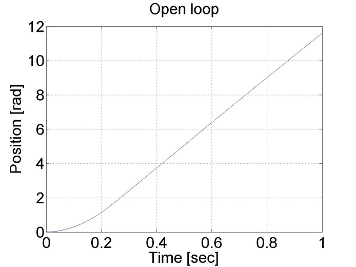
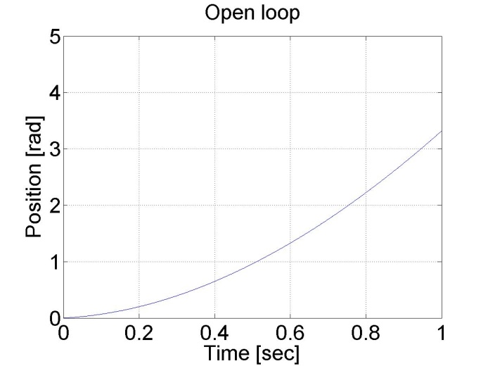
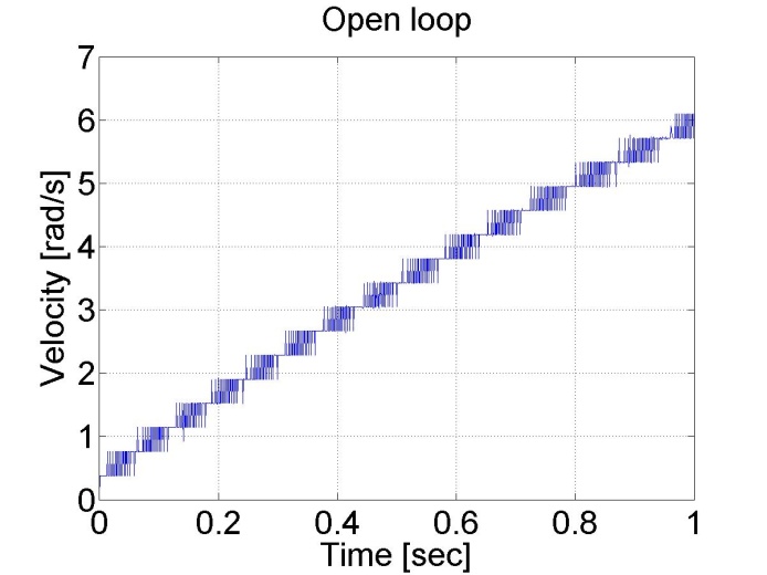
The results can be seen in the figure bellow. We can see that the position and the shaft speed diagram that the motor has a constant acceleration until it reaches its final shaft speed. The open loop control is very slow because of the constant voltage applied.

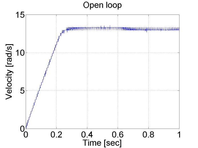
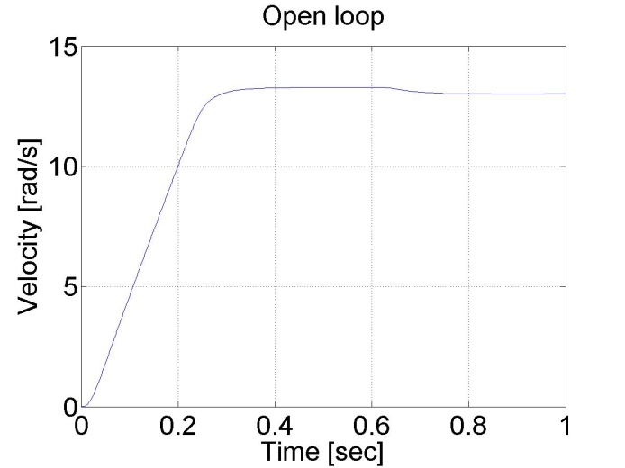
6.4.2. Task 2. Digital filter
The motor was tested with different output torque in this case. In the first case was applied 0.1 and 1 in the second case.
Measurement length in milliseconds: 1000
The state variable names:
-
time (given)
-
position (given)
-
velocity (given)
-
torque (given)
Declaration:
/* velocity filter variables */
static float  z_1=0.0, z_2=0.0, z_3=0.0;
static float ztmp_1=0.0, ztmp_2=0.0;
/* velocity filter parameters */
/* TSAMPLE=1e-3 and Tc=0.007 */
float ad11= 0.9996, ad12= 9.9072e-004, ad13= 4.3344e-007;
float ad21= -1.2637, ad22= 0.9730, ad23= 8.0496e-004;
float ad31= -2.3468e+003, ad32= -50.5468, ad33= 0.6280;
float bd1= 4.3671e-004, bd2= 1.2637, bd3= 2.3468e+003;
Controller:
/* Velocity filter  */
ztmp_1=ad11* z_1+ad12* z_2+ad13* z_3 + bd1* ResultData.Velocity;
ztmp_2=ad21* z_1+ad22* z_2+ad23* z_3 + bd2* ResultData.Velocity;
z_3=ad31* z_1+ad32* z_2+ad33* z_3 + bd3* ResultData.Velocity;
z_1  = ztmp_1;
z_2  = ztmp_2;
ResultData.Velocity =z_1;
ResultData.Torque = 1;
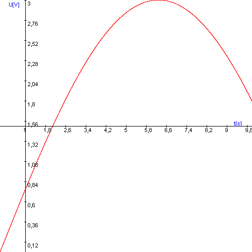
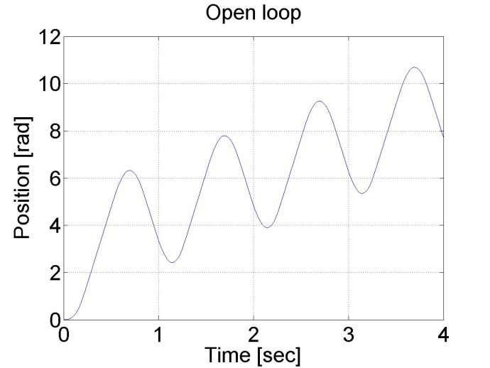
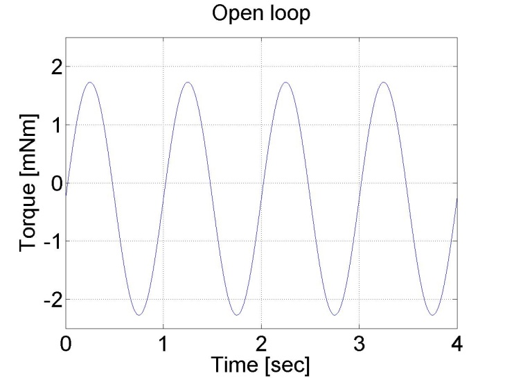
6.4.3. Task 3. Response of the motor to sinusoidal voltage and compensation of the servo amplifier offset
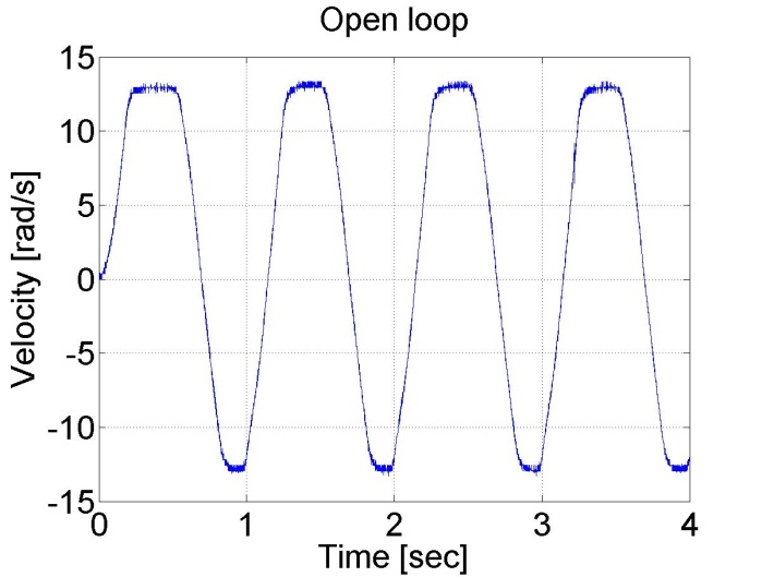
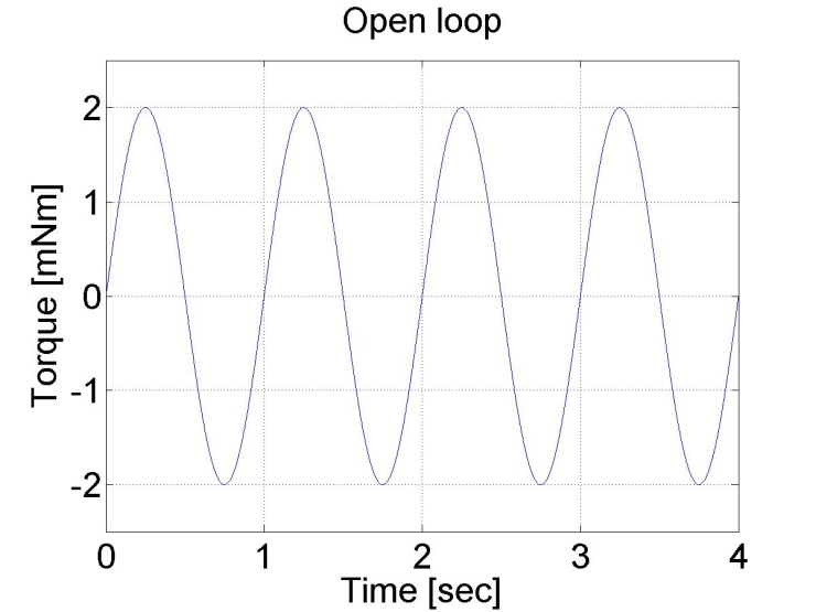
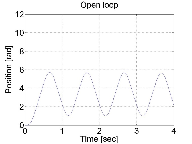
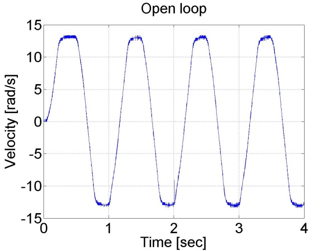
The servo amplifier of has an offset voltage. This is the most obvious if we apply a sinusoidal voltage. In this case we expect the motor to have sinusoidal shaft speed and sinusoidal position change coming from the shaft speed.
Measurement length in milliseconds : 4000
The state variable names:
-
time (given)
-
position (given)
-
velocity (given)
-
torque (given)
-
sin_torque (selected)
Declaration:
doubleparam = 0;
doublesinperiod = 1;
doublesinamplitude = 2;
doubleoffset = 0;
// please, change the offset in the range of -0.3 and -0.2
Controller:
// Current time in miliseconds
param = CurrentTime;
// Current time in seconds
param /= 1000;
// Result
param = param * 2 * PI / sinperiod;
//
// Controller part begin
//
// Sinusoidal voltage
ResultData.Torque = sinamplitude * sin(param) + offset;
ResultData.StateVariable_5 = sinamplitude * sin(param);
//
// Controller part end
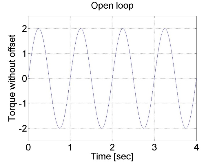
The results can be seen in the figure bellow. The position diagram is not pure sinusoidal, but it has a linear component too. This linear component is the offset of the servo amplifier. This can be subtracted from the applied voltage and this way the linear component in the position diagram disappears. The only change in the controller is in the declaration:
doubleoffset = -0.27;
The MATLAB program to plot the results
% please, modify it according to you file names
sv_1_14axc255hnyzli55axowlm55
sv_2_14axc255hnyzli55axowlm55
sv_3_14axc255hnyzli55axowlm55
sv_4_14axc255hnyzli55axowlm55
sv_5_14axc255hnyzli55axowlm55
time=time/1000;
plot(time,position)
set(gca, 'fontsize', [25]);
xlabel('Time [sec]');
ylabel('Position [rad]');
title('Open loop');
% you can adjust your axis
axis([0 4 0 12]);
grid
pause;
print -djpeg open_poz
plot(time,velocity)
set(gca, 'fontsize', [25]);
xlabel('Time [sec]');
ylabel('Velocity [rad/s]');
title('Open loop');
% you can adjust your axis
axis([0 4 -15 15]);
grid
print -djpeg open_vel
pause;
plot(time,torque)
set(gca, 'fontsize', [25]);
xlabel('Time [sec]');
ylabel('Torque [mNm]');
title('Open loop');
% you can adjust your axis
axis([0 4 -2.5 2.5]);
grid
print -djpeg open_torque
pause;
plot(time,sin_torque)
set(gca, 'fontsize', [25]);
xlabel('Time [sec]');
ylabel('Torque without offset');
title('Open loop');
% you can adjust your axis
axis([0 4 -2.5 2.5]);
grid
print -djpeg open_sin
|
|
|
|
|
|

(a)
|
|
|
|
|
|
(b)
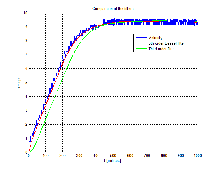
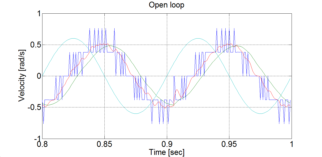
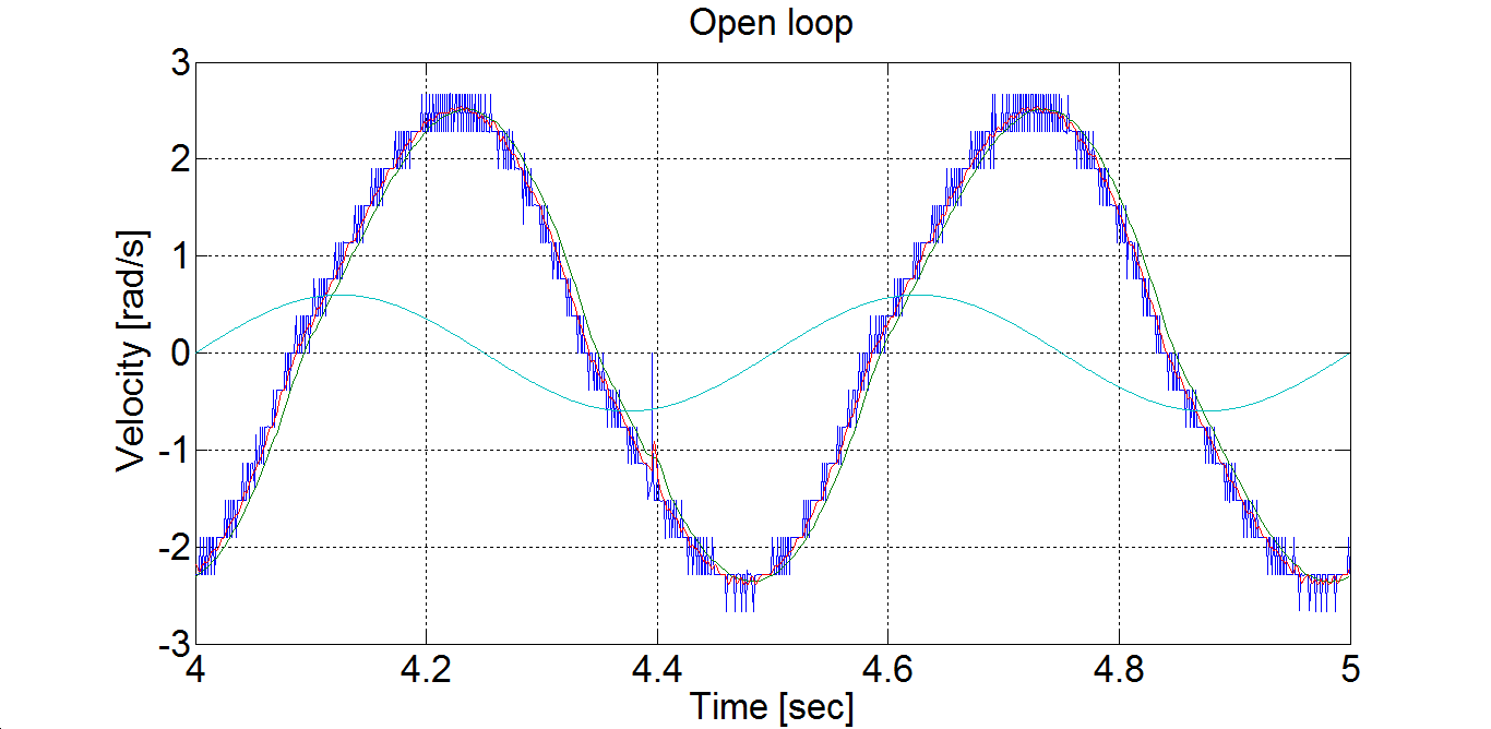
6.4.4. Comparison of digital filters
Measurement length in milliseconds : 4000
The state variable names:
-
time (given)
-
position (given)
-
velocity (given)
-
torque (given)
-
sin_torque (selected)
-
ref (selected)
-
filt (selected)
-
filtb (selected)
Declaration:
doubleparam = 0;
doublesinperiod = 0.1;
doublesinamplitude = 0.6;
doubleoffset = -0.217;
/* variables for filter */
static float  z_1=0.0, z_2=0.0, z_3=0.0;
static float ztmp_1=0.0, ztmp_2=0.0;
/* Tsample=1e-3  Tc=0.0032*/
float ad11 = 0.99591;
float ad12 = 0.00095987;
float ad13 = 3.652e-007;
float ad21 = -11.3235;
float ad22 = 0.88778;
float ad23 = 0.00061567;
float ad31 = -19089.6748;
float ad32 = -193.6165;
float ad33 = 0.30752;
float bd1  = 0.0040906;
float bd2  = 11.3235;
float bd3  = 19089.6748;
/* Variables for Bessel filter */
static float  z_1b=0.0, z_2b=0.0, z_3b=0.0;
static float ztmp_1b=0.0, ztmp_2b=0.0;
/* Bessel Tsample=1e-3  Tc=0.0032*/
float ad11b = 0.95193;
float ad12b = 0.00083371;
float ad13b = 2.6009e-007;
float ad21b = -120.9668;
float ad22b = 0.56688;
float ad23b = 0.00034345;
float ad31b = -159737.83;
float ad32b = -629.4281;
float ad33b = -0.080513;
float bd1b  = 0.048071;
float bd2b  = 120.9668;
float bd3b  = 159737.83;
Controller:
// Current time
param = CurrentTime;
// Only milliseconds
param /= 1000;
// Result
param = param * 2 * PI / sinperiod;
//
// Controller part begin
//
// Sinusoidal voltage
ResultData.Torque = sinamplitude * sin(param) + offset;
ResultData.StateVariable_5 = sinamplitude * sin(param);
/* Velocity filter  */
ztmp_1=ad11* z_1+ad12* z_2+ad13* z_3 + bd1* ResultData.Velocity;
ztmp_2=ad21* z_1+ad22* z_2+ad23* z_3 + bd2* ResultData.Velocity;
z_3=ad31* z_1+ad32* z_2+ad33* z_3 + bd3* ResultData.Velocity;
z_1  = ztmp_1;
z_2  = ztmp_2;
ResultData.StateVariable_6=z_1;
/* Bessel velocity filter  */
ztmp_1b=ad11b* z_1b+ad12b* z_2b+ad13b* z_3b + bd1b* ResultData.Velocity;
ztmp_2b=ad21b* z_1b+ad22b* z_2b+ad23b* z_3b + bd2b* ResultData.Velocity;
z_3b=ad31b* z_1b+ad32b* z_2b+ad33b* z_3b + bd3b* ResultData.Velocity;
z_1b  = ztmp_1b;
z_2b  = ztmp_2b;
ResultData.StateVariable_7=z_1b;
Measurement with two different frequency
doublesinperiod = 0.1;
and
doublesinperiod = 0.5;
The steady state are plotted in Figure 6-1 and Figure 6-2
The MATLAB program for generating Figure 6-1 and Figure 6-2
sv_1_zlwzmf45pqyn1c45p31cvve4
sv_2_zlwzmf45pqyn1c45p31cvve4
sv_3_zlwzmf45pqyn1c45p31cvve4
sv_4_zlwzmf45pqyn1c45p31cvve4
sv_5_zlwzmf45pqyn1c45p31cvve4
sv_6_zlwzmf45pqyn1c45p31cvve4
sv_7_zlwzmf45pqyn1c45p31cvve4

plot(time,velocity,time,filt,time,filtb,time,ref)
set(gca, 'fontsize', [25]);
xlabel('Time [sec]');
ylabel('Velocity [rad/s]');
title('Open loop');
% you can adjust your axis
% axis([0.8 1 -1 1]);
axis([4 5 -3 3]);
grid
print -djpeg open_vel
6.5. Closed Loop Control Measurements -- Exercise 5
6.5.1. Parameter tuning of the P controller -- Test 1.
The first task in PID control is to tune the parameters of the controller. For this we used the Ziegler-Nichols method which is easy to implement empirically for the system even for a beginner in control theory. In the figure bellow the Ziegler-Nichols tuning chart can be seen.
|
AP |
I |
TD |
|
|
P control |
AU/2 |
||
|
PI control |
AU/2.2 |
1.2AP/Tu |
|
|
PID control zó |
AU/1.7 |
2AP/Tu |
AP Tu/8 |
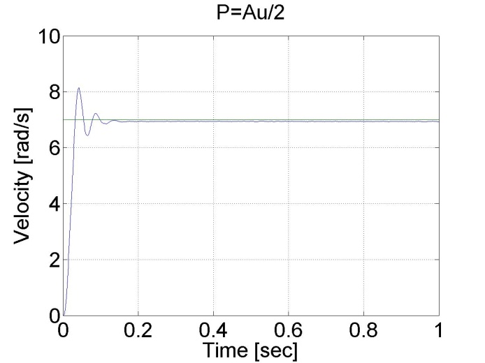
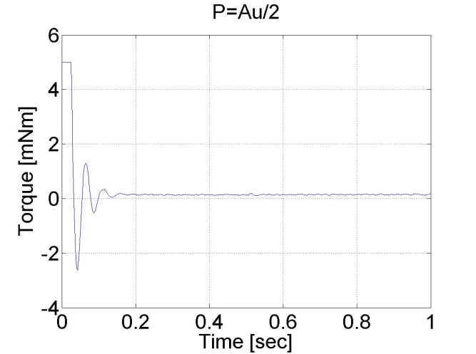
The first step in the tuning is to create a P controller with arbitrary AU value. The controller has the following form:
Measurement length in milliseconds: 1000
The state variable names:
-
time (given)
-
position (given)
-
velocity (given)
-
torque (given)
-
ref (selected)
-
error (selected)
Declaration:
doubleP = 4.75;
doubleref_vel = 7;
doubleerror_vel= 0;
/* velocity filter variables */
static float  z_1=0.0, z_2=0.0, z_3=0.0;
static float ztmp_1=0.0, ztmp_2=0.0;
/* velocity filter parameters */
/* TSAMPLE=1e-3 and Tc=0.005 */
float ad11= 0.9989, ad12= 9.8248e-004, ad13= 4.0937e-007;
float ad21= -3.2749, ad22= 0.9497, ad23= 7.3686e-004;
float ad31= -5.8949e+003, ad32= -91.6978, ad33= 0.5076;
float bd1= 0.0011, bd2= 3.2749, bd3= 5.8949e+003;
Controller:
/* Velocity filter  */
ztmp_1=ad11* z_1+ad12* z_2+ad13* z_3 + bd1* ResultData.Velocity;
ztmp_2=ad21* z_1+ad22* z_2+ad23* z_3 + bd2* ResultData.Velocity;
z_3=ad31* z_1+ad32* z_2+ad33* z_3 + bd3* ResultData.Velocity;
z_1  = ztmp_1;
z_2  = ztmp_2;
 ResultData.Velocity =z_1;
//Error calculation for velocity control
error_vel=ref_vel- ResultData.Velocity;
ResultData.StateVariable_5 = ref_vel;
ResultData.StateVariable_6 = error_vel;
ResultData.Torque = P*error_vel;
if (ResultData.Torque > 5)
{
ResultData.Torque = 5;
}
if (ResultData.Torque < -5)
{
ResultData.Torque = -5;
}
The controller also sets the minimal and maximal values of the output voltage to 5 and -5 V. The results can be seen in the figure bellow.
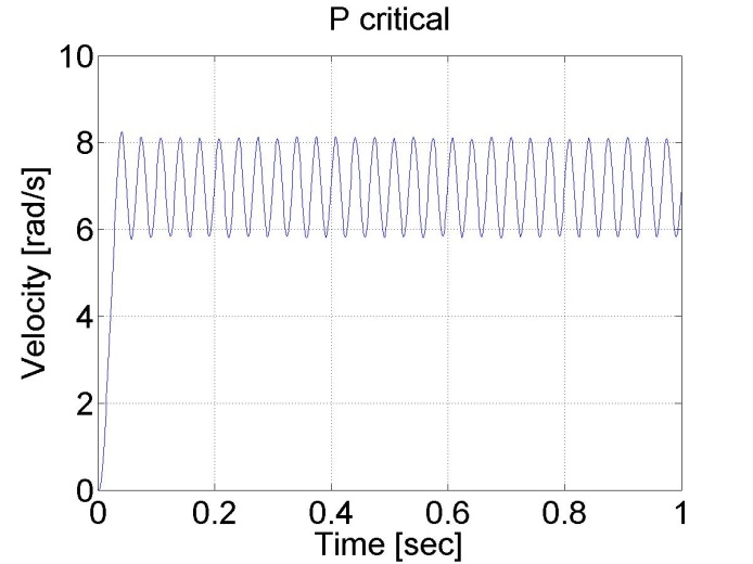
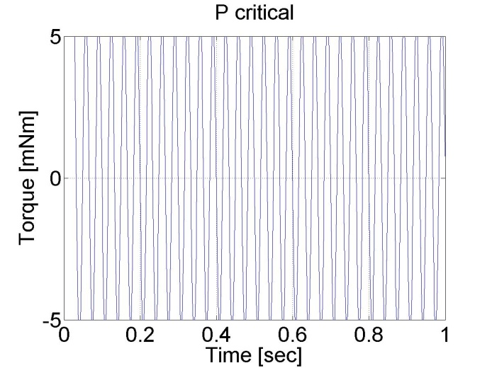
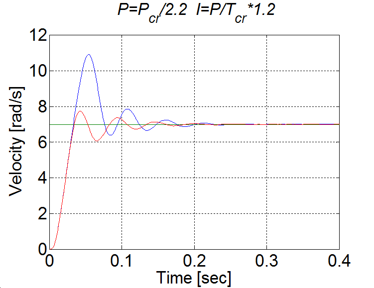
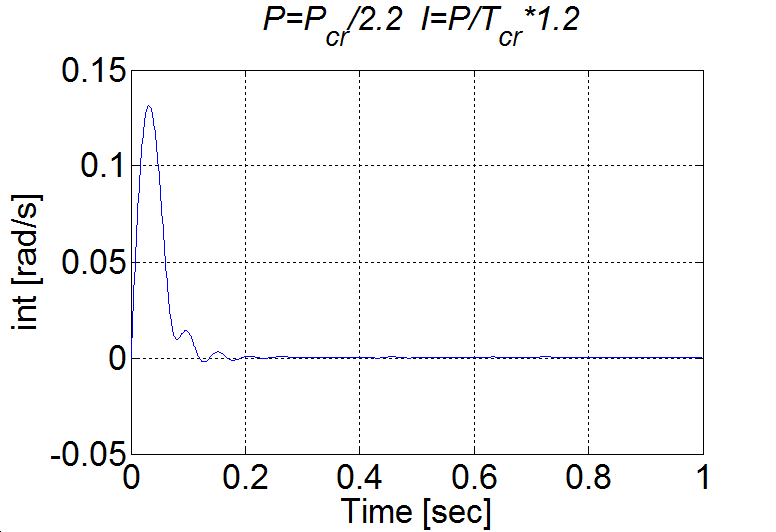
We can conclude that AU = 4.75 and TU≈0.2/6. According to the table PPI=2.1 and IPI=75.
Remark!!! the values of AU and TU depend on the filter parameter.
6.5.2. Step signal response of the P controller -- Test 2.
For this test we set the reference shaft speed to 1 rad/s. The controller has the following form:
Enter measurement length in milliseconds: 1000
The state variable names:
-
time (given)
-
position (given)
-
velocity (given)
-
torque (given)
-
ref (selected)
-
error (selected)
-
integral (selected)
Declaration:
doubleP_par = 2.3;
doubleI_par = 0.0;
doubleref_vel = 7;
doubleerror_vel;
static doubleerror_vel_int=0.0;
double load = 0;
/* velocity filter variables */
static float z_1=0.0, z_2=0.0, z_3=0.0;
static float ztmp_1=0.0, ztmp_2=0.0;
/* TSAMPLE=1e-3 and Tc=0.0027 */
float ad11= 0.9936, ad12= 9.4621e-004, ad13= 3.4524e-007;
float ad21= - 17.5400, ad22= 0.8515, ad23= 5.6261e-004;
float ad31= -2.8584e+004, ad32= -249.0676, ad33= 0.2264;
float bd1= 0.0064, bd2= 17.5400, bd3= 2.8584e+004;
Controller:
/* Velocity filter */
ztmp_1=ad11* z_1+ad12* z_2+ad13* z_3 + bd1* ResultData.Velocity;
ztmp_2=ad21* z_1+ad22* z_2+ad23* z_3 + bd2* ResultData.Velocity;
z_3=ad31* z_1+ad32* z_2+ad33* z_3 + bd3* ResultData.Velocity;
z_1 = ztmp_1;
z_2 = ztmp_2;
ResultData.Velocity =z_1;
//Error calculation for velocity control
error_vel=ref_vel- ResultData.Velocity;
error_vel_int = error_vel_int + error_vel*(CurrentTime - OldTime)/1000;
ResultData.StateVariable_5 = ref_vel;
ResultData.StateVariable_6 = error_vel;
ResultData.StateVariable_7 = error_vel_int;
ResultData.Torque = P_par*error_vel + I_par*error_vel_int - load;
if (ResultData.Torque > 5) { ResultData.Torque = 5; }
if (ResultData.Torque < -5) { ResultData.Torque = -5; }
The results can be seen in the figure bellow. We can see that the P controller has a constant error in steady state.
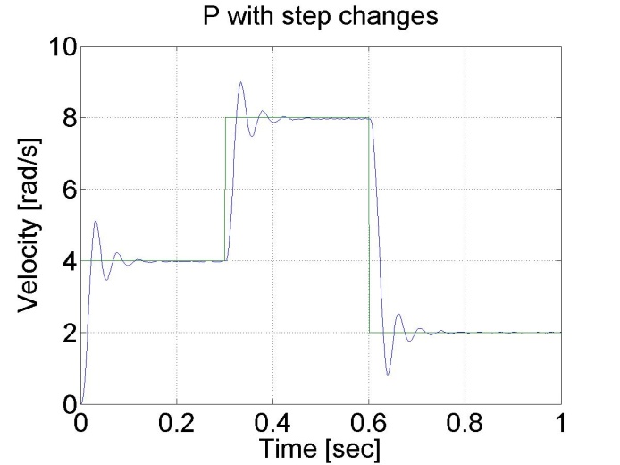
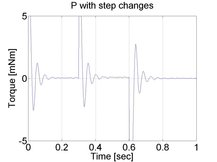
6.5.3. Response of the P controller to step changes in the reference speed signal -- Test 3.
In this test the reference shaft speed changed in two time instances, at t = 0.2 s and at t = 0.4 s. The constant error of the P controller is noticeable in this case too. The controller has the following form:
Enter measurement length in milliseconds: 1000
The state variable names:
-
time (given)
-
position (given)
-
velocity (given)
-
torque (given)
-
ref (selected)
-
error (selected)
-
integral (selected)
Declaration:
doubleP_par = 2.3;
doubleI_par = 0.0;
doubleref_vel = 7;
doubleerror_vel;
static doubleerror_vel_int=0.0;
double load = 0;
/* velocity filter variables */
static float z_1=0.0, z_2=0.0, z_3=0.0;
static float ztmp_1=0.0, ztmp_2=0.0;
/* TSAMPLE=1e-3 and Tc=0.0027 */
float ad11= 0.9936, ad12= 9.4621e-004, ad13= 3.4524e-007;
float ad21= - 17.5400, ad22= 0.8515, ad23= 5.6261e-004;
float ad31= -2.8584e+004, ad32= -249.0676, ad33= 0.2264;
float bd1= 0.0064, bd2= 17.5400, bd3= 2.8584e+004;
Controller:
//Step changes in reference speed
if (CurrentTime > 0*1e3 && CurrentTime < 0.2*1e3)
{
ref_vel = 4;
}
if (CurrentTime >= 0.2*1e3 && CurrentTime < 0.4*1e3)
{
ref_vel = 8;
}
if (CurrentTime >= 0.4*1e3 && CurrentTime < 0.6*1e3)
{
ref_vel = 2;
}
/* Velocity filter */
ztmp_1=ad11* z_1+ad12* z_2+ad13* z_3 + bd1* ResultData.Velocity;
ztmp_2=ad21* z_1+ad22* z_2+ad23* z_3 + bd2* ResultData.Velocity;
z_3=ad31* z_1+ad32* z_2+ad33* z_3 + bd3* ResultData.Velocity;
z_1 = ztmp_1;
z_2 = ztmp_2;
ResultData.Velocity =z_1;
//Error calculation for velocity control
error_vel=ref_vel- ResultData.Velocity;
error_vel_int = error_vel_int + error_vel*(CurrentTime - OldTime)/1000;
ResultData.StateVariable_5 = ref_vel;
ResultData.StateVariable_6 = error_vel;
ResultData.StateVariable_7 = error_vel_int;
ResultData.Torque = P_par*error_vel + I_par*error_vel_int - load;
if (ResultData.Torque > 5) { ResultData.Torque = 5; }
if (ResultData.Torque < -5) { ResultData.Torque = -5; }
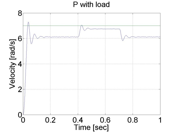
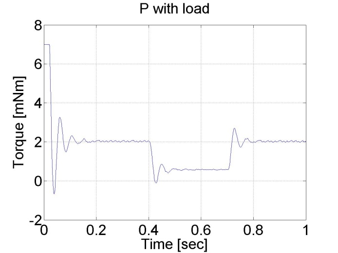
6.5.4. Response of the P controller to step changes in the load -- Test 4.
We can see the largest drawback of the P controller that it has a constant error and it is not able to reject disturbances.
Enter measurement length in milliseconds: 1000
The state variable names :
-
time (given)
-
position (given)
-
velocity (given)
-
torque (given)
-
ref (selected)
-
error (selected)
-
integral (selected)
Declaration:
doubleP_par = 2.3;
doubleI_par = 0.0;
doubleref_vel = 7;
doubleerror_vel;
static doubleerror_vel_int=0.0;
double load = 2;
/* velocity filter variables */
static float z_1=0.0, z_2=0.0, z_3=0.0;
static float ztmp_1=0.0, ztmp_2=0.0;
/* TSAMPLE=1e-3 and Tc=0.0027 */
float ad11= 0.9936, ad12= 9.4621e-004, ad13= 3.4524e-007;
float ad21= - 17.5400, ad22= 0.8515, ad23= 5.6261e-004;
float ad31= -2.8584e+004, ad32= -249.0676, ad33= 0.2264;
float bd1= 0.0064, bd2= 17.5400, bd3= 2.8584e+004;
Controller:
if (CurrentTime >= 0.4*1e3 && CurrentTime < 0.7*1e3)
{
load = 0.5;
}
/* Velocity filter */
ztmp_1=ad11* z_1+ad12* z_2+ad13* z_3 + bd1* ResultData.Velocity;
ztmp_2=ad21* z_1+ad22* z_2+ad23* z_3 + bd2* ResultData.Velocity;
z_3=ad31* z_1+ad32* z_2+ad33* z_3 + bd3* ResultData.Velocity;
z_1 = ztmp_1;
z_2 = ztmp_2;
ResultData.Velocity =z_1;
//Error calculation for velocity control
error_vel=ref_vel- ResultData.Velocity;
error_vel_int = error_vel_int + error_vel*(CurrentTime - OldTime)/1000;
ResultData.StateVariable_5 = ref_vel;
ResultData.StateVariable_6 = error_vel;
ResultData.StateVariable_7 = error_vel_int;
ResultData.Torque = P_par*error_vel + I_par*error_vel_int - load;
if (ResultData.Torque > 5) { ResultData.Torque = 5; }
if (ResultData.Torque < -5) { ResultData.Torque = -5; }
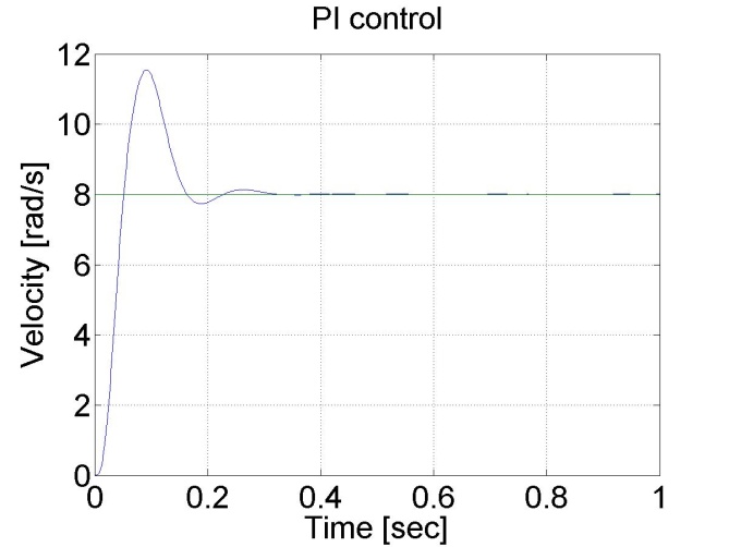
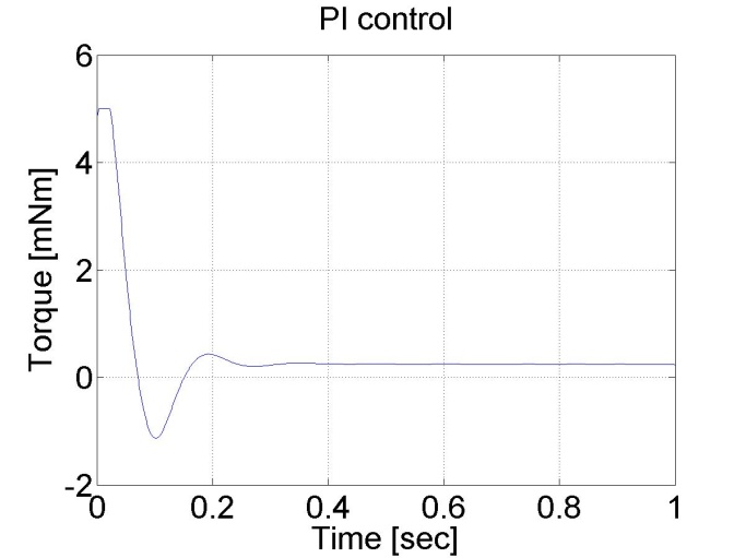
6.5.5. Step signal response of the PI controller -- Test 2.
For this test we set the reference shaft speed to 1 rad/s. The controller has the following form:
Enter measurement length in milliseconds: 1000
The state variable names:
-
time (given)
-
position (given)
-
velocity (given)
-
torque (given)
-
ref (selected)
-
error (selected)
-
integral (selected)
Declaration:
doubleP = 0.6;
doubleI = 7;
doubleref_vel = 8;
doubleerror_vel;
static doubleerror_vel_int=0.0;
double load = 0;
/* velocity filter variables */
static float z_1=0.0, z_2=0.0, z_3=0.0;
static float ztmp_1=0.0, ztmp_2=0.0;
/* velocity filter parameters */
/* TSAMPLE=1e-3 and Tc=0.007 */
float ad11= 0.9996, ad12= 9.9072e-004, ad13= 4.3344e-007;
float ad21= -1.2637, ad22= 0.9730, ad23= 8.0496e-004;
float ad31= -2.3468e+003, ad32= -50.5468, ad33= 0.6280;
float bd1= 4.3671e-004, bd2= 1.2637, bd3= 2.3468e+003;
Controller:
/* Velocity filter */
ztmp_1=ad11* z_1+ad12* z_2+ad13* z_3 + bd1* ResultData.Velocity;
ztmp_2=ad21* z_1+ad22* z_2+ad23* z_3 + bd2* ResultData.Velocity;
z_3=ad31* z_1+ad32* z_2+ad33* z_3 + bd3* ResultData.Velocity;
z_1 = ztmp_1;
z_2 = ztmp_2;
ResultData.Velocity =z_1;
//Error calculation for velocity control
error_vel=ref_vel- ResultData.Velocity;
error_vel_int = error_vel_int + error_vel*(CurrentTime - OldTime)/1000.0;
ResultData.StateVariable_5 = ref_vel;
ResultData.StateVariable_6 = error_vel;
ResultData.StateVariable_7 = error_vel_int;
ResultData.StateVariable_8 = CurrentTime;
ResultData.Torque = P*error_vel + I*error_vel_int - load;
if (ResultData.Torque > 5)
{
ResultData.Torque = 5;
}
if (ResultData.Torque < -5)
{
ResultData.Torque = -5;
}
The noticeable difference from the P controller is the lack of steady state error. This is the effect of the integral part of the controller, which summarizes the error. The integral error is also presented, which has a large value at the beginning and decreases afterwards. The PI controller is also faster form the P controller. Its drawback is, that is can lead to large overshot or even to instability. This can be eliminated by adding a D element to the controller.
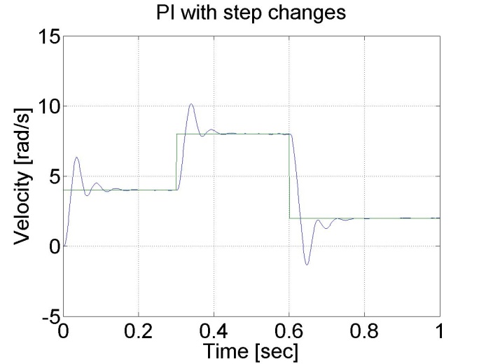
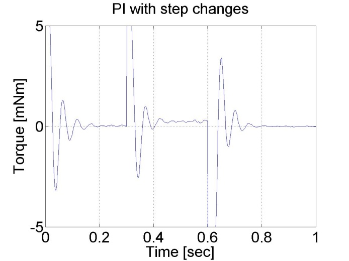
6.5.6. Response of the PI controller to step changes in the reference speed signal -- Test 3.
In this test the reference shaft speed changed in two time instances, at t = 0.3 s and at t = 0.6 s. The PI controller is faster compared to the P controller and the motor operates without steady state error. The controller has the following form:
Enter measurement length in milliseconds: 1000
The state variable names:
-
time (given)
-
position (given)
-
velocity (given)
-
torque (given)
-
ref (selected)
-
error (selected)
-
integral (selected)
Declaration:
doubleP_par = 2;
doubleI_par = 50.0;
doubleref_vel = 7;
doubleerror_vel;
static doubleerror_vel_int=0.0;
double load = 0;
/* velocity filter variables */
static float z_1=0.0, z_2=0.0, z_3=0.0;
static float ztmp_1=0.0, ztmp_2=0.0;
/* TSAMPLE=1e-3 and Tc=0.0027 */
float ad11= 0.9936, ad12= 9.4621e-004, ad13= 3.4524e-007;
float ad21= - 17.5400, ad22= 0.8515, ad23= 5.6261e-004;
float ad31= -2.8584e+004, ad32= -249.0676, ad33= 0.2264;
float bd1= 0.0064, bd2= 17.5400, bd3= 2.8584e+004;
Controller:
//Step changes in reference speed
if (CurrentTime > 0*1e3 && CurrentTime < 0.3*1e3)
{
ref_vel = 4;
}
if (CurrentTime >= 0.3*1e3 && CurrentTime < 0.6*1e3)
{
ref_vel = 8;
}
if (CurrentTime >= 0.6*1e3 && CurrentTime < 1.6*1e3)
{
ref_vel = 2;
}
/* Velocity filter */
ztmp_1=ad11* z_1+ad12* z_2+ad13* z_3 + bd1* ResultData.Velocity;
ztmp_2=ad21* z_1+ad22* z_2+ad23* z_3 + bd2* ResultData.Velocity;
z_3=ad31* z_1+ad32* z_2+ad33* z_3 + bd3* ResultData.Velocity;
z_1 = ztmp_1;
z_2 = ztmp_2;
ResultData.Velocity =z_1;
//Error calculation for velocity control
error_vel=ref_vel- ResultData.Velocity;
error_vel_int = error_vel_int + error_vel*(CurrentTime - OldTime)/1000;
ResultData.StateVariable_5 = ref_vel;
ResultData.StateVariable_6 = error_vel;
ResultData.StateVariable_7 = error_vel_int;
ResultData.Torque = P_par*error_vel + I_par*error_vel_int - load;
if (ResultData.Torque > 5) { ResultData.Torque = 5; }
if (ResultData.Torque < -5) { ResultData.Torque = -5; }
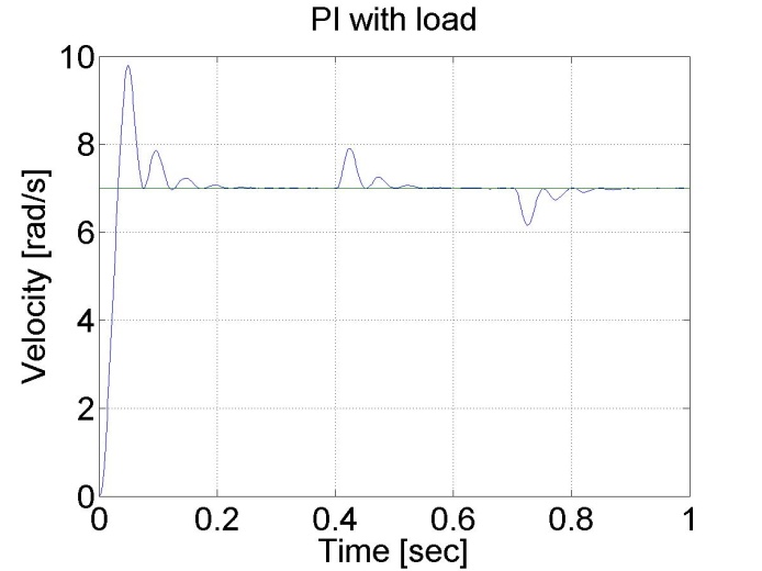
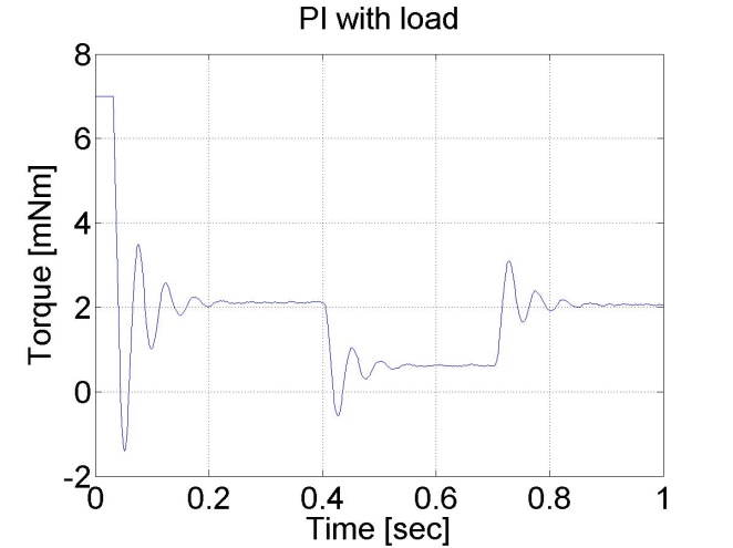
6.5.7. Response of the PI controller to step changes in the load -- Test 4.
In this test, a constant virtual load is added if t < 0.3 s than load=2.0 load, if 0.3 s<t < 0.7 s than load=0.5 finally if t >0.7 s than load=2.0 again.
Enter measurement length in milliseconds: 1000
The state variable names:
-
time (given)
-
position (given)
-
velocity (given)
-
torque (given)
-
ref (selected)
-
error (selected)
-
integral (selected)
Declaration:
doubleP_par = 2.3;
doubleI_par = 50;
doubleref_vel = 7;
doubleerror_vel;
static doubleerror_vel_int=0.0;
double load = 2;
/* velocity filter variables */
static float z_1=0.0, z_2=0.0, z_3=0.0;
static float ztmp_1=0.0, ztmp_2=0.0;
/* TSAMPLE=1e-3 and Tc=0.0027 */
float ad11= 0.9936, ad12= 9.4621e-004, ad13= 3.4524e-007;
float ad21= - 17.5400, ad22= 0.8515, ad23= 5.6261e-004;
float ad31= -2.8584e+004, ad32= -249.0676, ad33= 0.2264;
float bd1= 0.0064, bd2= 17.5400, bd3= 2.8584e+004;
Controller:
/* Velocity filter */
ztmp_1=ad11* z_1+ad12* z_2+ad13* z_3 + bd1* ResultData.Velocity;
ztmp_2=ad21* z_1+ad22* z_2+ad23* z_3 + bd2* ResultData.Velocity;
z_3=ad31* z_1+ad32* z_2+ad33* z_3 + bd3* ResultData.Velocity;
z_1 = ztmp_1;
z_2 = ztmp_2;
ResultData.Velocity =z_1;
if (CurrentTime >= 0.4*1e3 && CurrentTime < 0.7*1e3)
{
load = 0.5;
}
//Error calculation for velocity control
error_vel=ref_vel- ResultData.Velocity;
error_vel_int = error_vel_int + error_vel*(CurrentTime - OldTime)/1000.0;
ResultData.StateVariable_5 = ref_vel;
ResultData.StateVariable_6 = error_vel;
ResultData.StateVariable_7 = error_vel_int;
ResultData.Torque = P_par*error_vel + I_par*error_vel_int - load;
if (ResultData.Torque > 5)
{
ResultData.Torque = 5;
}
if (ResultData.Torque < -5)
{
ResultData.Torque = -5;
}
We can notice that the PI controller is good at disturbance rejection on the contrary to the P controller.
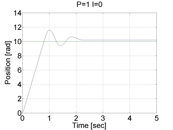
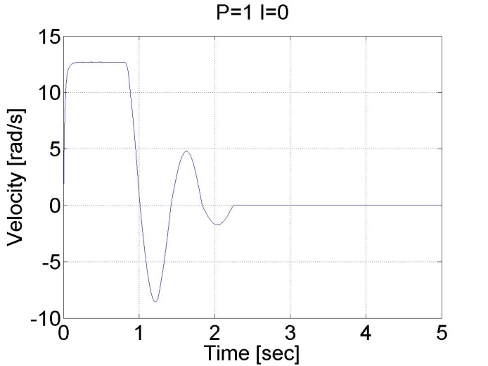
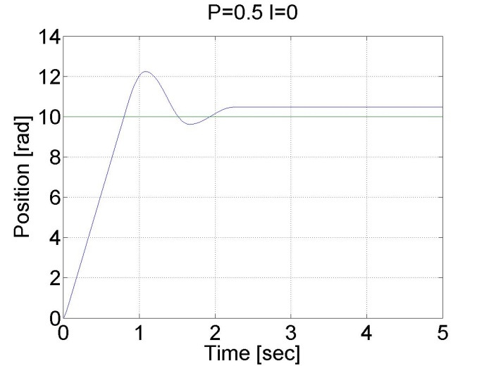
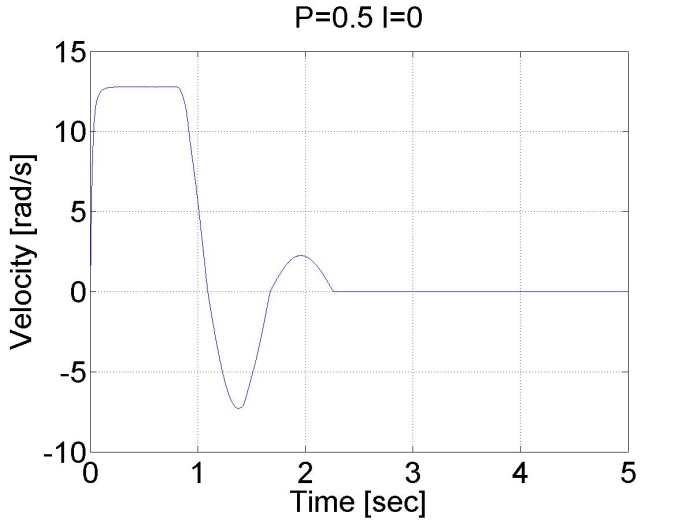
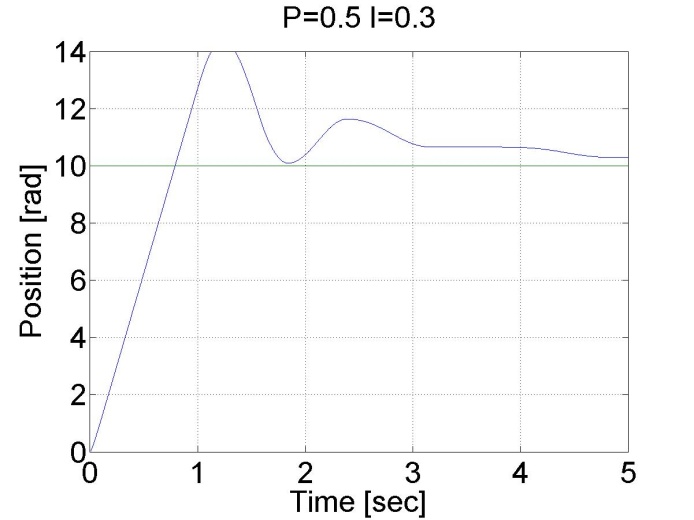
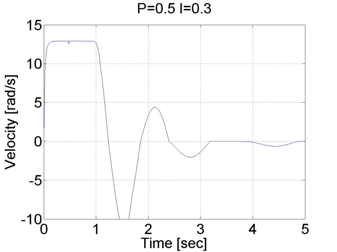
6.5.8. Step signal response of the P and PI controller -- Test 1.
For this test we set the reference shaft position to 10 rad. The controller has the following form:
Enter measurement length in milliseconds: 1000
The state variable names:
-
time (given)
-
position (given)
-
velocity (given)
-
torque (given)
-
ref (selected)
-
error (selected)
-
integral (selected)
Declaration:
doubleP_par = 1;
doubleI_par = 0;
doubleref_pos = 10;
doubleerror_pos;
static doubleerror_pos_int=0.0;
double load = 0;
/* velocity filter variables */
static float z_1=0.0, z_2=0.0, z_3=0.0;
static float ztmp_1=0.0, ztmp_2=0.0;
/* TSAMPLE=1e-3 and Tc=0.0027 */
float ad11= 0.9936, ad12= 9.4621e-004, ad13= 3.4524e-007;
float ad21= - 17.5400, ad22= 0.8515, ad23= 5.6261e-004;
float ad31= -2.8584e+004, ad32= -249.0676, ad33= 0.2264;
float bd1= 0.0064, bd2= 17.5400, bd3= 2.8584e+004;
static double ini_0 = 0;
static double ini_1 = -10;
Controller:
if (ini_1 < 0)
{
ini_0 = ResultData.Position;
}
ini_1 = 5;
/* Velocity filter */
ztmp_1=ad11* z_1+ad12* z_2+ad13* z_3 + bd1* ResultData.Velocity;
ztmp_2=ad21* z_1+ad22* z_2+ad23* z_3 + bd2* ResultData.Velocity;
z_3=ad31* z_1+ad32* z_2+ad33* z_3 + bd3* ResultData.Velocity;
z_1 = ztmp_1;
z_2 = ztmp_2;
ResultData.Velocity =z_1;
//Error calculation for velocity control
error_pos=ref_pos- ResultData.Position + ini_0;
error_pos_int = error_pos_int + error_pos*(CurrentTime - OldTime)/1000.0;
ResultData.StateVariable_5 = ref_pos;
ResultData.StateVariable_6 = error_pos;
ResultData.StateVariable_7 = error_pos_int;
ResultData.StateVariable_8 = ResultData.Position - ini_0;
ResultData.Torque = P_par*error_pos + I_par*error_pos_int - load;
if (ResultData.Torque > 5)
{
ResultData.Torque = 5;
}
if (ResultData.Torque < -5)
{
ResultData.Torque = -5;
}
We can see that there is a large overshot in this controller, and the steady state error is also present. On the other hand, the position is measured and not calculated by derivation, the position curve is smooth compared to the shaft speed curves in the previous cases.
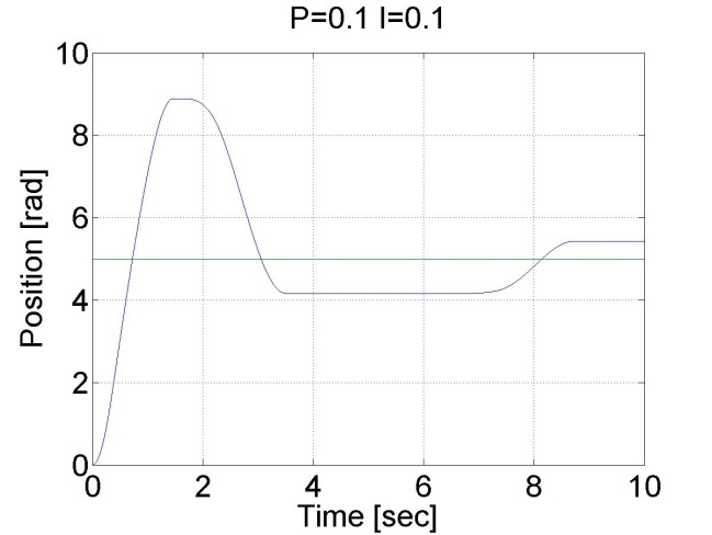
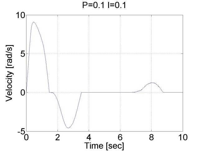
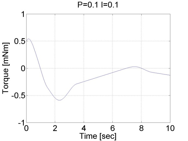
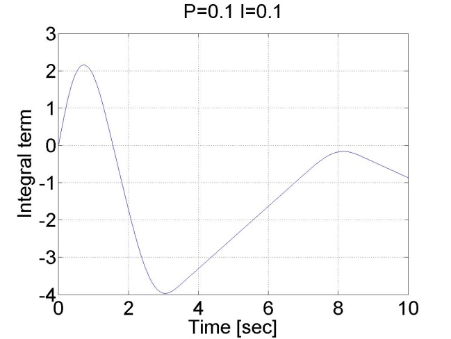
6.5.9. Stick-slip phenomenon
Enter measurement length in milliseconds: 10000
The state variable names:
-
time (given)
-
position (given)
-
velocity (given)
-
torque (given)
-
ref (selected)
-
error (selected)
-
integral (selected)
Declaration:
doubleP_par = 0.1;
doubleI_par = 0.1;
doubleref_pos = 5;
doubleerror_pos;
static doubleerror_pos_int=0.0;
double load = 0;
/* velocity filter variables */
static float z_1=0.0, z_2=0.0, z_3=0.0;
static float ztmp_1=0.0, ztmp_2=0.0;
/* TSAMPLE=1e-3 and Tc=0.0027 */
float ad11= 0.9936, ad12= 9.4621e-004, ad13= 3.4524e-007;
float ad21= - 17.5400, ad22= 0.8515, ad23= 5.6261e-004;
float ad31= -2.8584e+004, ad32= -249.0676, ad33= 0.2264;
float bd1= 0.0064, bd2= 17.5400, bd3= 2.8584e+004;
static double ini_0 = 0;
static double ini_1 = -10;
Controller:
if (ini_1 < 0)
{
ini_0 = ResultData.Position;
}
ini_1 = 5;
/* Velocity filter */
ztmp_1=ad11* z_1+ad12* z_2+ad13* z_3 + bd1* ResultData.Velocity;
ztmp_2=ad21* z_1+ad22* z_2+ad23* z_3 + bd2* ResultData.Velocity;
z_3=ad31* z_1+ad32* z_2+ad33* z_3 + bd3* ResultData.Velocity;
z_1 = ztmp_1;
z_2 = ztmp_2;
ResultData.Velocity =z_1;
//Error calculation for velocity control
error_pos=ref_pos- CurrentPosition;
error_pos_int = error_pos_int + error_pos*(CurrentTime - OldTime)/1000.0;
ResultData.StateVariable_5 = ref_pos;
ResultData.StateVariable_6 = error_pos;
ResultData.StateVariable_7 = error_pos_int;
ResultData.Torque = P_par*error_pos + I_par*error_pos_int - load;
if (ResultData.Torque > 5)
{
ResultData.Torque = 5;
}
if (ResultData.Torque < -5)
{
ResultData.Torque = -5;
}
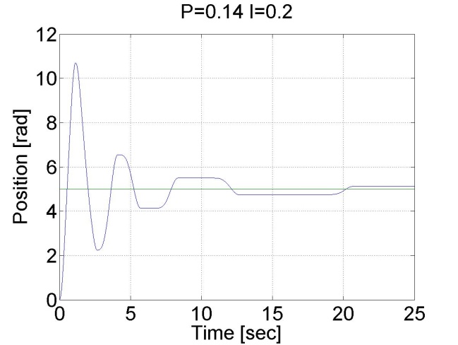
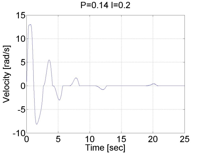
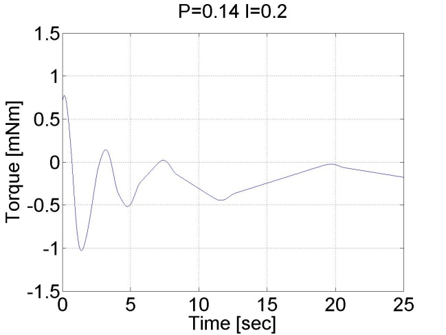
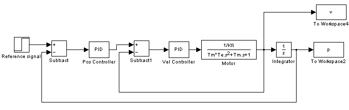
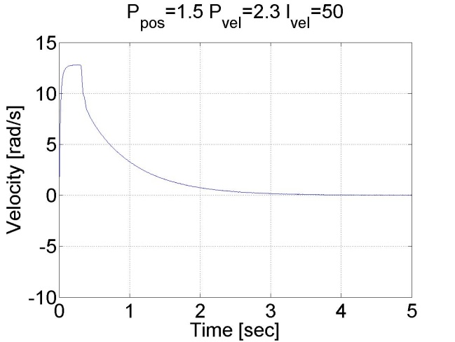
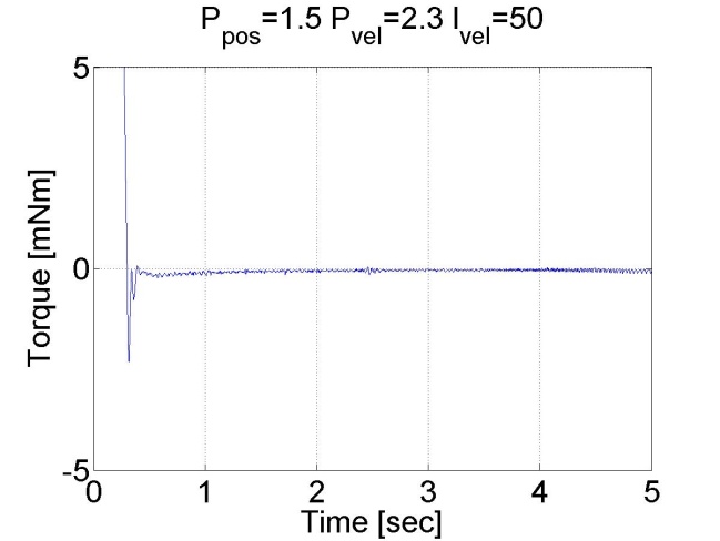
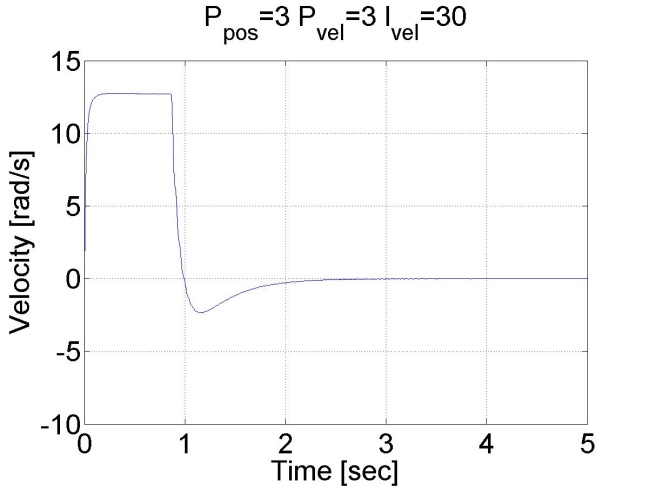
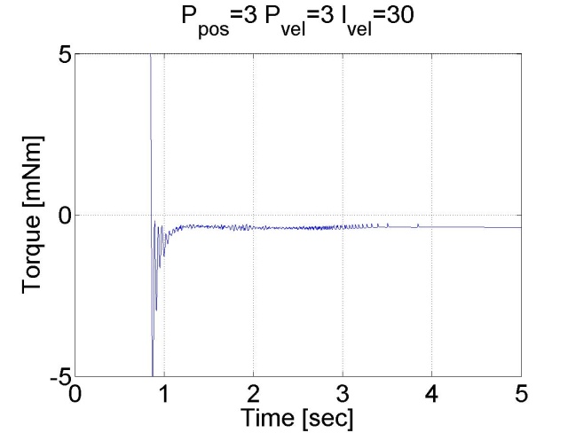
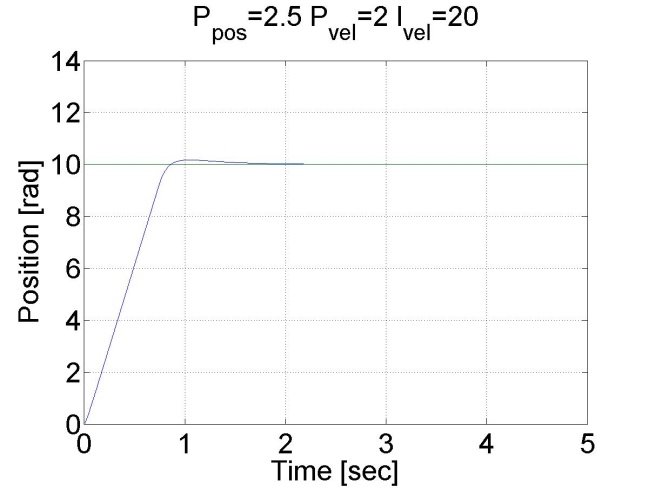
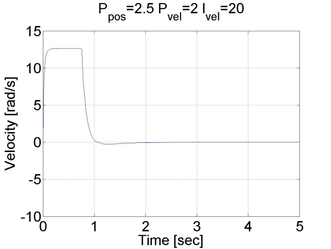
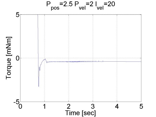
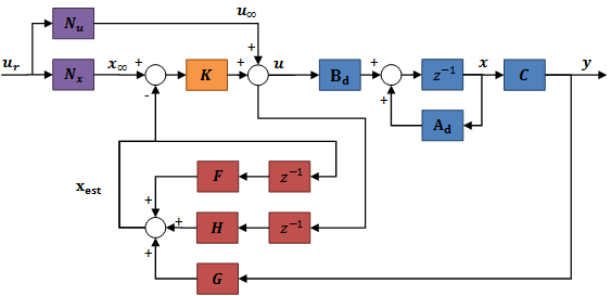
6.5.10. Step signal response of the position controller with inner shaft speed controller -- Test 1.
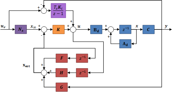
The motor reached the reference position. The reason for the overshot is that it takes time to decelerate the motor. This effect can be eliminated if we introduce an inner control loop for the shaft speed of the motor. The reference value for the shaft speed is coming from the position error of the motor, this means that as the motor reaches its reference position the reference shaft speed starts do decrease. The reference shaft speed is almost zero if the motor is close to the reference position. The structure of this controller can be seen in the figure bellow. The position controller is P type and the shaft speed controller is PI type.
The controller code is the following:
The state variable names:
-
time (given)
-
position (given)
-
velocity (given)
-
torque (given)
-
ref_poz (selected)
-
ref_vel (selected)
-
err_pos (selected)
-
err_vel (selected)
-
int_vel (selected)
-
poz (selected)
Declaration:
doubleP_pos = 3;
doubleP_vel = 3;
doubleI_vel = 30;
doubleref_pos = 10;
doubleref_vel = 0;
doubleerror_pos = 0;
doubleerror_vel = 0;
static doubleerror_vel_int = 0;
static doubleini_0 = 0;
static doubleini_1 = -10;
/* velocity filter variables */
static float z_1=0.0, z_2=0.0, z_3=0.0;
static float ztmp_1=0.0, ztmp_2=0.0;
/* TSAMPLE=1e-3 and Tc=0.0027 */
float ad11= 0.9936, ad12= 9.4621e-004, ad13= 3.4524e-007;
float ad21= - 17.5400, ad22= 0.8515, ad23= 5.6261e-004;
float ad31= -2.8584e+004, ad32= -249.0676, ad33= 0.2264;
float bd1= 0.0064, bd2= 17.5400, bd3= 2.8584e+004;
Controller:
if (ini_1 < 0)
{
ini_0 = ResultData.Position;
}
ini_1 = 5;
/* Velocity filter */
ztmp_1=ad11* z_1+ad12* z_2+ad13* z_3 + bd1* ResultData.Velocity;
ztmp_2=ad21* z_1+ad22* z_2+ad23* z_3 + bd2* ResultData.Velocity;
z_3=ad31* z_1+ad32* z_2+ad33* z_3 + bd3* ResultData.Velocity;
z_1 = ztmp_1;
z_2 = ztmp_2;
ResultData.Velocity =z_1;
//Error calculation for position control
error_pos = ref_pos- ResultData.Position + ini_0;
// Error calculation for velocity control
ref_vel = error_pos*P_pos;
error_vel = ref_vel - ResultData.Velocity;
error_vel_int = error_vel_int + error_vel*(CurrentTime - OldTime)/1000;
ResultData.StateVariable_5 = ref_pos;
ResultData.StateVariable_6 = ref_vel;
ResultData.StateVariable_7 = error_pos;
ResultData.StateVariable_8 = error_vel;
ResultData.StateVariable_9 = error_vel_int;
ResultData.StateVariable_10 = ResultData.Position - ini_0;
//Controller
ResultData.Torque = P_vel*error_vel + I_vel*error_vel_int;
if (ResultData.Torque > 5)
{
ResultData.Torque = 5;
}
if (ResultData.Torque < -5)
{
ResultData.Torque = -5;
}
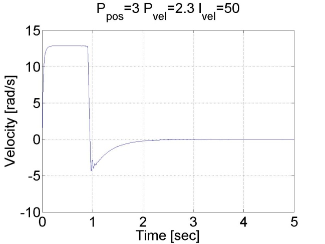
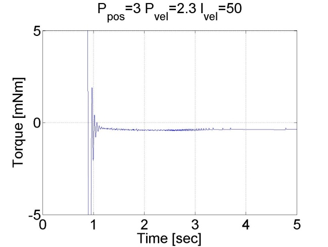
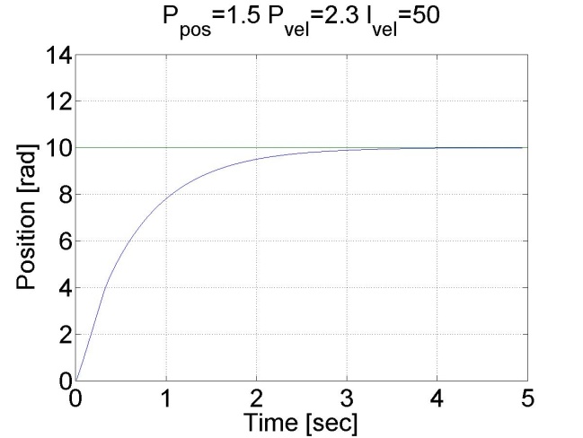
We can see that there is no overshot in this case, because the shaft speed starts decreasing in time. We can conclude that position control with inner shaft speed control loop gives much better results than the simple P position controller.


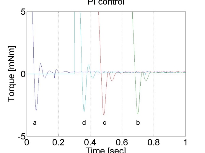
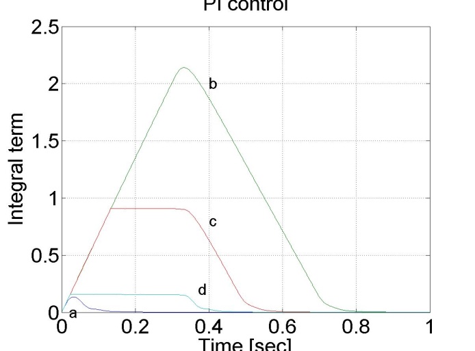
6.5.11. Fault tolerance measurements
Enter measurement length in milliseconds: 1000
The state variable names:
-
time (given)
-
position (given)
-
velocity (given)
-
torque (given)
-
ref (selected)
-
error (selected)
-
integral (selected)
Declaration:
doubleP_par = 2;
doubleI_par = 50;
doubleref_vel = 7;
doubleerror_vel;
static doubleerror_vel_int=0.0;
double load = 0;
/*
// in case of a
doubleint_lim = 100;
doubleTf = -0.3*1e3;
// in case of b
doubleint_lim = 100;
doubleTf = 0.3*1e3;
// in case of c
doubleint_lim = 0.9;
doubleTf = 0.3*1e3;
// in case of d
doubleint_lim = 0.15;
doubleTf = 0.3*1e3;
*/
// Please, copy one of the above pair of parameters
doubleint_lim = 0.15;
doubleTf = 0.3*1e3;
Controller:
/* velocity filter variables */
static float z_1=0.0, z_2=0.0, z_3=0.0;
static float ztmp_1=0.0, ztmp_2=0.0;
/* TSAMPLE=1e-3 and Tc=0.0027 */
float ad11= 0.9936, ad12= 9.4621e-004, ad13= 3.4524e-007;
float ad21= - 17.5400, ad22= 0.8515, ad23= 5.6261e-004;
float ad31= -2.8584e+004, ad32= -249.0676, ad33= 0.2264;
float bd1= 0.0064, bd2= 17.5400, bd3= 2.8584e+004;
/* Velocity filter */
ztmp_1=ad11* z_1+ad12* z_2+ad13* z_3 + bd1* ResultData.Velocity;
ztmp_2=ad21* z_1+ad22* z_2+ad23* z_3 + bd2* ResultData.Velocity;
z_3=ad31* z_1+ad32* z_2+ad33* z_3 + bd3* ResultData.Velocity;
z_1 = ztmp_1;
z_2 = ztmp_2;
ResultData.Velocity =z_1;
//Error calculation for velocity control
error_vel=ref_vel- ResultData.Velocity;
error_vel_int = error_vel_int + error_vel*(CurrentTime - OldTime)/1000.0;
ResultData.StateVariable_5 = ref_vel;
ResultData.StateVariable_6 = error_vel;
ResultData.StateVariable_7 = error_vel_int;
if (error_vel_int > int_lim)
{
error_vel_int = int_lim;
}
ResultData.Torque = P_par*error_vel + I_par*error_vel_int - load;
if ( CurrentTime < Tf)
{
ResultData.Torque = 0.0;
}
if (ResultData.Torque > 5)
{
ResultData.Torque = 5;
}
if (ResultData.Torque < -5)
{
ResultData.Torque = -5;
}
Enter measurement length in milliseconds: 1000
The state variable names:
-
time (given)
-
position (given)
-
velocity (given)
-
torque (given)
-
ref (selected)
-
error (selected)
-
integral (selected)
Declaration:
doubleP_par = 2.1;
doubleI_par = 75.0;
doubleref_vel = 7;
doubleerror_vel;
static doubleerror_vel_int=0.0;
double load = 2;
double delta = 0;
/* velocity filter variables */
static float z_1=0.0, z_2=0.0, z_3=0.0;
static float ztmp_1=0.0, ztmp_2=0.0;
/* Tsample=1e-3 and Tc=0.0027 */
float ad11= 0.9936, ad12= 9.4621e-004, ad13= 3.4524e-007;
float ad21= - 17.5400, ad22= 0.8515, ad23= 5.6261e-004;
float ad31= -2.8584e+004, ad32= -249.0676, ad33= 0.2264;
float bd1= 0.0064, bd2= 17.5400, bd3= 2.8584e+004;
Controller:
/* Velocity filter */
ztmp_1=ad11* z_1+ad12* z_2+ad13* z_3 + bd1* ResultData.Velocity;
ztmp_2=ad21* z_1+ad22* z_2+ad23* z_3 + bd2* ResultData.Velocity;
z_3=ad31* z_1+ad32* z_2+ad33* z_3 + bd3* ResultData.Velocity;
z_1 = ztmp_1;
z_2 = ztmp_2;
ResultData.Velocity =z_1;
//Error calculation for velocity control
error_vel=ref_vel- ResultData.Velocity;
delta=error_vel*(CurrentTime - OldTime)/1000;
error_vel_int = error_vel_int + delta;
ResultData.StateVariable_5 = ref_vel;
ResultData.StateVariable_6 = error_vel;
ResultData.Torque = P_par*error_vel + I_par*error_vel_int - load;
if (ResultData.Torque > 5) { ResultData.Torque = 5; error_vel_int = error_vel_int - delta*0; }
if (ResultData.Torque < -5) { ResultData.Torque = -5; error_vel_int = error_vel_int - delta*0;}
ResultData.StateVariable_7 = error_vel_int;
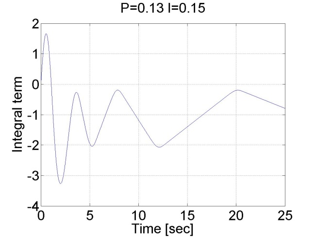
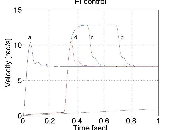
The oveshoot can be reduced by switching off the integrator term during controller saturation
Comparision of the integral terms in two cases
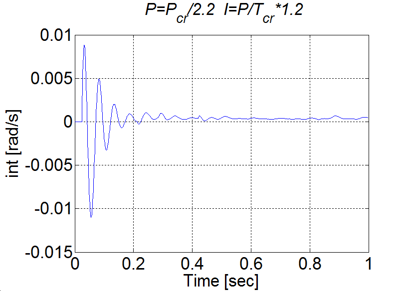
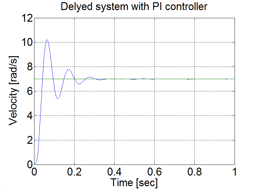
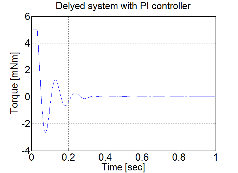
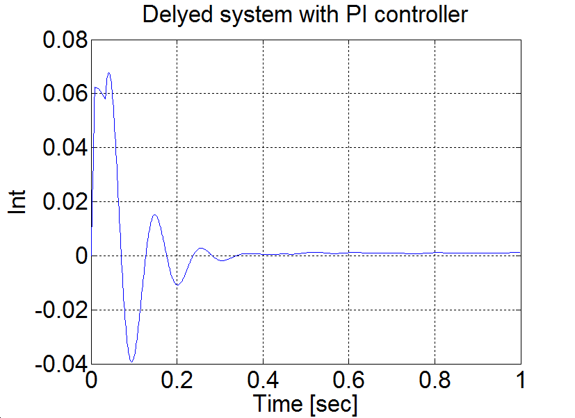
6.5.12. Control of time-delay system
Enter measurement length in milliseconds: 1000
The state variable names:
-
time (given)
-
position (given)
-
velocity (given)
-
torque (given)
-
ref (selected)
-
error (selected)
-
integral (selected)
Declaration:
doubleP_par = 0.85;
doubleI_par = 12.0;
doubleref_vel = 7;
doubleerror_vel;
static doubleerror_vel_int=0.0;
double load = 0;
/* Time delay pipe */
static float T_1=0.0, T_2=0.0, T_3=0.0;
static float T_4=0.0, T_5=0.0, T_6=0.0;
static float T_7=0.0, T_8=0.0, T_9=0.0;
/* velocity filter variables */
static float z_1=0.0, z_2=0.0, z_3=0.0;
static float ztmp_1=0.0, ztmp_2=0.0;
/* Tsample=1e-3 and Tc=0.0032 */
float ad11 = 0.99591, ad12 = 0.00095987, ad13 = 3.652e-007;
float ad21 = -11.3235, ad22 = 0.88778, ad23 = 0.00061567;
float ad31 = -19089.6748, ad32 = -193.6165, ad33 = 0.30752;
float bd1 = 0.0040906, bd2 = 11.3235, bd3 = 19089.6748;
Controller:
//Step changes in reference speed
/* Velocity filter */
ztmp_1=ad11* z_1+ad12* z_2+ad13* z_3 + bd1* ResultData.Velocity;
ztmp_2=ad21* z_1+ad22* z_2+ad23* z_3 + bd2* ResultData.Velocity;
z_3=ad31* z_1+ad32* z_2+ad33* z_3 + bd3* ResultData.Velocity;
z_1 = ztmp_1;
z_2 = ztmp_2;
ResultData.Velocity =z_1;
//Error calculation for velocity control
error_vel=ref_vel- ResultData.Velocity;
error_vel_int = error_vel_int + error_vel*(CurrentTime - OldTime)/1000;
ResultData.StateVariable_5 = ref_vel;
ResultData.StateVariable_6 = error_vel;
ResultData.StateVariable_7 = error_vel_int;
ResultData.Torque = T_1;
T_1=T_2;
T_2=T_3;
T_3=T_4;
T_4=T_5;
T_5=T_6;
T_6=T_7;
T_7=T_8;
T_8=T_9;
T_9= P_par*error_vel + I_par*error_vel_int - load;
if (T_9 > 5) { T_9 = 5;
error_vel_int = error_vel_int - error_vel*(CurrentTime - OldTime)/1000;}
if (T_9 < -5) { T_9 = -5;
error_vel_int = error_vel_int - error_vel*(CurrentTime - OldTime)/1000;}
Az eredményeket megjelenítő MATLAB program
% please, modify it according to you file names
sv_1_hwztupv131qjbi55l3k5oi45
sv_2_hwztupv131qjbi55l3k5oi45
sv_3_hwztupv131qjbi55l3k5oi45
sv_4_hwztupv131qjbi55l3k5oi45
sv_5_hwztupv131qjbi55l3k5oi45
sv_6_hwztupv131qjbi55l3k5oi45
sv_7_hwztupv131qjbi55l3k5oi45
time=time/1000;
plot(time,position)
set(gca, 'fontsize', [25]);
xlabel('Time [sec]');
ylabel('Position [rad]');
title('Delyed system with PI controller');
% you can adjust your axis
axis([0 1 0 12]);
grid
pause;
print -djpeg Delay_poz
plot(time,velocity)
set(gca, 'fontsize', [25]);
xlabel('Time [sec]');
ylabel('Velocity [rad/s]');
title('Delyed system with PI controller');
% you can adjust your axis
axis([0 1 0 12]);
grid
print -djpeg Delay_vel
pause;
plot(time,torque)
set(gca, 'fontsize', [25]);
xlabel('Time [sec]');
ylabel('Torque [mNm]');
title('Delyed system with PI controller');
% you can adjust your axis
%axis([0 1 -1 1]);
grid
print -djpeg Delay_torque
pause;
plot(time,int)
set(gca, 'fontsize', [25]);
xlabel('Time [sec]');
ylabel('Int');
title('Delyed system with PI controller');
% you can adjust your axis
%axis([0 1 -1 1]);
grid
print -djpeg Delay_int
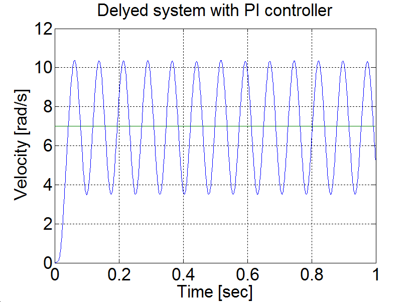
Conclusion AU = 1.7 and TU≈0.08. According to the table PPI=0.85 and IPI=12. Measurement results are shown in Figure 6-7.
P control results
6.5.13. Sliding mode control results
Sliding mode control can be also applied. There are two different measurements. The control part of the measurements is the same, but since the velocity of the motor is calculated from position data, this makes the velocity diagram noisy. By applying a filter for the velocity the results are smoother.
Enter measurement length in milliseconds: 12000
The state variable names:
-
time (given)
-
position (given)
-
velocity (given)
-
torque (given)
-
sigma (selected)
The controller code is the following:
Declaration:
float sigma;
float error;
float error_dot;
float ref=5.0;
float lambda=2;
static double ini_0 = 0;
static double ini_1 = -10;
Controller:
if (ini_1 < 0)
{
ini_0 = ResultData.Position;
}
ini_1 = 5;
error=ref-ResultData.Position+ ini_0;
error_dot=- ResultData.Velocity;
sigma= error+ lambda*error_dot;
ResultData.StateVariable_5 = sigma;
if (sigma>0)
{ ResultData.Torque=0.1;
}
if (sigma<0)
{ ResultData.Torque =-0.1;
}
if (sigma=0)
{ ResultData.Torque=0;
}
Select item to download: All files
Please, download them by clicking the button “DOWNLOAD”
The results are plotted by the following MATLAB file:
% please, modify it according to you file names
sv_1_n0ktqaui51tw5hrtvpypxu45
sv_2_n0ktqaui51tw5hrtvpypxu45
sv_3_n0ktqaui51tw5hrtvpypxu45
sv_4_n0ktqaui51tw5hrtvpypxu45
sv_5_n0ktqaui51tw5hrtvpypxu45
time=time/1000;
plot(time,position)
set(gca, 'fontsize', [25]);
xlabel('Time [sec]');
ylabel('Position [rad]');
title('Sliding mode controller');
% you can adjust your axis
axis([0 12 0 6]);
grid
pause;
print -djpeg smc_poz
plot(time,velocity)
set(gca, 'fontsize', [25]);
xlabel('Time [sec]');
ylabel('Velocity [rad/s]');
title('Sliding mode controller');
% you can adjust your axis
axis([0 12 0 3]);
grid
print -djpeg smc_vel
pause;
plot(5-position,-velocity)
set(gca, 'fontsize', [25]);
xlabel('Position error [rad]');
ylabel('Velocity error [rad/s]');
title('Sliding mode controller');
% you can adjust your axis
axis([0 5 -3 0]);
grid
print -djpeg smc_traj
pause;
plot(time,torque)
set(gca, 'fontsize', [25]);
xlabel('Time [sec]');
ylabel('Torque [mNm]');
title('Sliding mode controller');
% you can adjust your axis
axis([0 12 -0.15 0.15]);
grid
print -djpeg smc_torque
pause;
plot(time,sigma)
set(gca, 'fontsize', [25]);
xlabel('Time [sec]');
ylabel('Sigma');
title('Sliding mode controller');
% you can adjust your axis
axis([0 12 -2.5 2.5]);
grid
print -djpeg smc_sigm
|
|
|
|
|
|
|
|
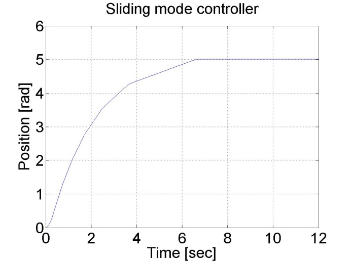
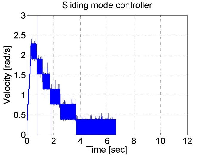
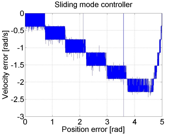
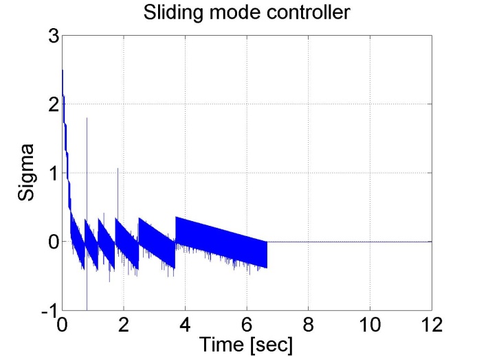
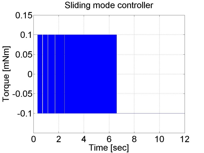
Figure 6-16. Results of the position controller with sliding mode controller
The sliding mode controller with the velocity filter has the following form:
Declaration:
float sigma;
float error;
float error_dot;
float ref=5.0;
float lambda=2;
/* filter variables*/
static float z_1=0.0, z_2=0.0, z_3=0.0;
static float ztmp_1=0.0, ztmp_2=0.0;
/*omega_c=10 unmodelled dynamics of the filter causes big chattering */
float Azd11= 1, Azd12= 0.0010, Azd13= 0.0000;
float Azd21= -0.0005, Azd22= 0.9999, Azd23= 0.0010;
float Azd31= -0.9851, Azd32= -0.2960, Azd33= 0.9703;
float Bzd1= 0.0000, Bzd2= 0.0005, Bzd3= 0.9851;
/* omega_c= 1/0.007 unmodelled dynamics of the filter does not cause big chattering
float Azd11= 0.9996, Azd12= 9.9072e-004, Azd13= 4.3344e-007;
float Azd21= -1.2637, Azd22= 0.9730, Azd23= 8.0496e-004;
float Azd31= -2.3468e+003, Azd32= -50.5468, Azd33= 0.6280;
float Bzd1= 4.3671e-004, Bzd2= 1.2637, Bzd3= 2.3468e+003;
*/
static double ini_0 = 0;
static double ini_1 = -10;
Controller:
if (ini_1 < 0)
{
ini_0 = ResultData.Position;
}
ini_1 = 5;
error=ref-ResultData.Position+ ini_0;
/* filter */
ztmp_1 = Azd11* z_1 +Azd12* z_2 +Azd13* z_3 + Bzd1*ResultData.Velocity ;
ztmp_2 = Azd21* z_1 +Azd22* z_2 +Azd23* z_3 + Bzd2*ResultData.Velocity ;
z_3 = Azd31*z_1 +Azd32*z_2 +Azd33* z_3 + Bzd3*ResultData.Velocity ;
z_1 = ztmp_1;
z_2 = ztmp_2;
ResultData.Velocity =z_1;
error_dot=- z_1;
sigma=error+ lambda*error_dot;
ResultData.StateVariable_5 = sigma;
if (sigma>0)
{ ResultData.Torque=0.1;}
if (sigma<0)
{ ResultData.Torque =-0.1;
}
if (sigma=0)
{ ResultData.Torque=0;}
The results can be seen in the figure below:
|
|
|
|
|
|
|
|

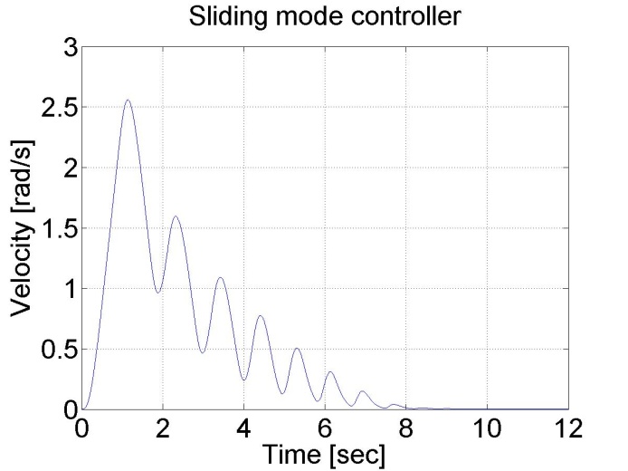
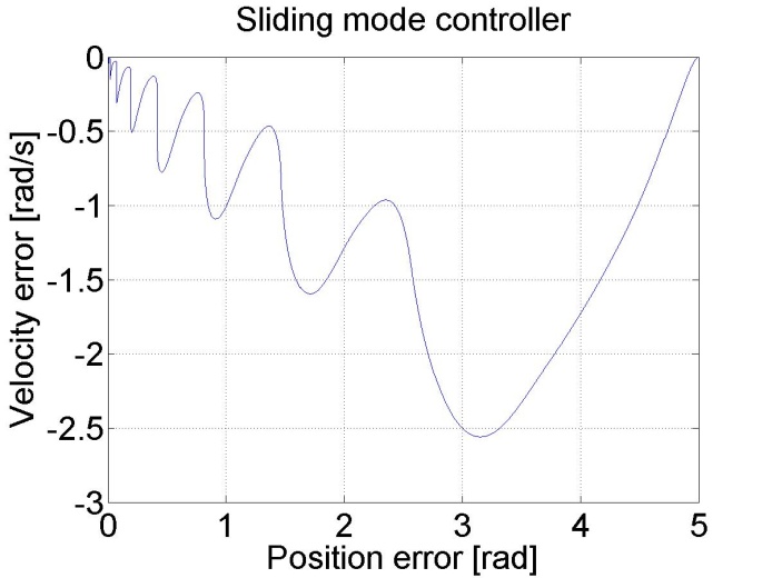
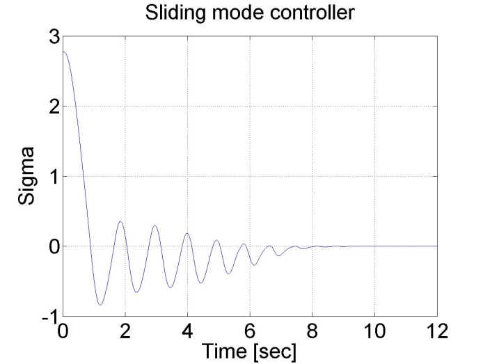
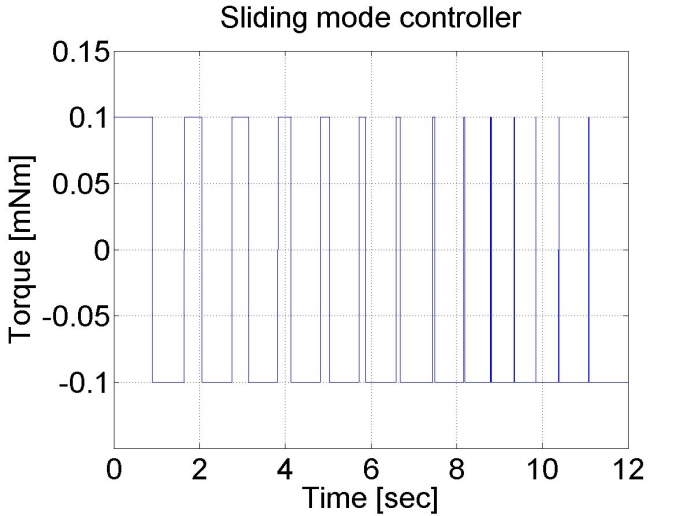
Figure 6-16. Sliding mode control with a velocity filter
|
|
|
|
|
|
|
|
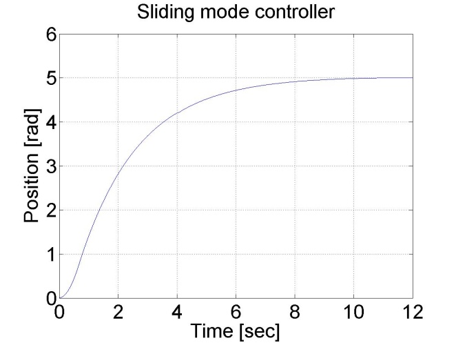
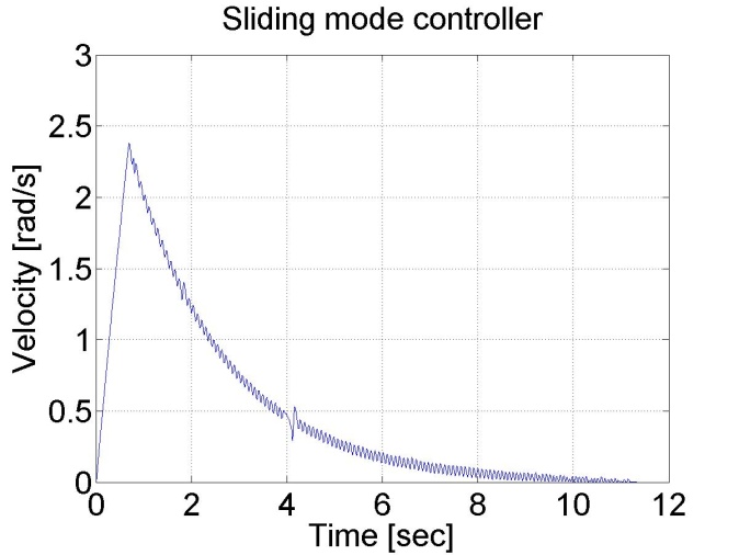
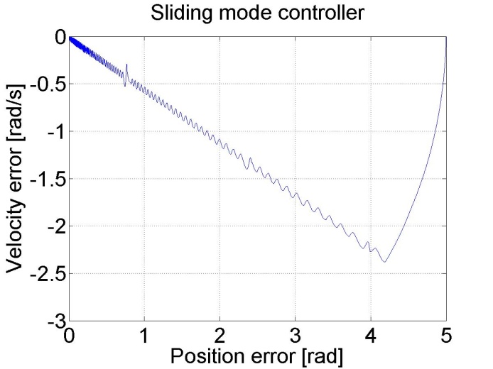
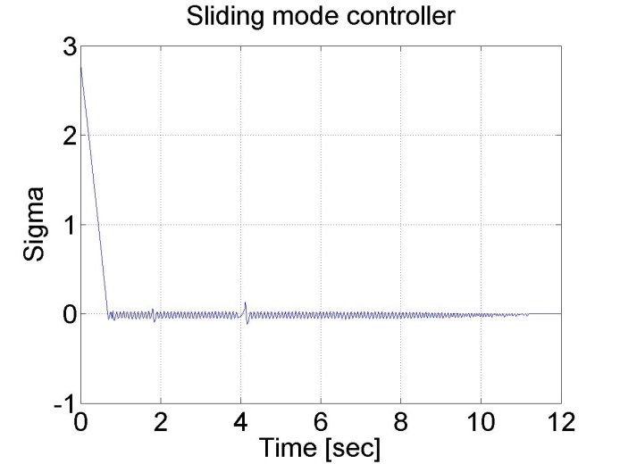
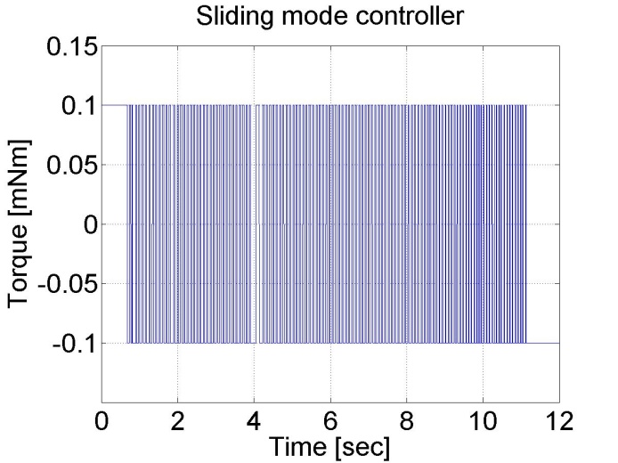
Figure 6-17. Results of the position controller with sliding mode controller with velocity filter
6.6. Complex design and measurement
In this section the theoretical basics of the DC motor control will be reviewed by focusing on the state feedback control. As the control of the motor is solved by a computer, the model expressed in discretized form. Furthermore the introduced methods will be implemented into MATLAB. In the theoretical review, only the necessary steps for implementation is emphasized. The more detailed description of methods can be found in the recommended literature.
6.6.1. State feedback and its design
Let us consider the following explicit Discrete time invariant state space model:
|
|
(6.1) |
Where
-

: the state vector at k
-

: the column vector of the input signal at k
-

: the vector of the output signal at k,
-

: the system matrix,
-

: the input matrix,
-

: the output matrix,
-

: feedthrough matrix (usually 0),
The purpose of state feedback is to change the system matrix in a way that the behaviour of the system is favourable to us. Since the eigenvalues of  are the system’s poles, it is evident, that by changing the eigenvalues we can manipulate the behaviour of the system freely (with particular limits). From the state space equations it can be seen that if we choose
  to:
to:
|
|
(6.2) |
then the value of  can be changed.
Thus we get:
|
|
(6.3) |

Where:
-

: the feedback matrix
-

: the new input signal of the system,
The new system matrix is  , which value can be set with
  . Since K does not affect the system matrix directly - but after the multiplication with
  – it is not possible to have an arbitrary result.
Hence the condition for design and correct operation of a state feedback is the controllability of the system represented by the state space model. This means that the system can reach any state – with the proper input signal – from any given state in a finite interval. In case of a Discrete time system the condition of total state controllability is that the rank of controllability matrix  of the system is equal to the number of state variables (n):
|
|
(6.4) |

Designing the state feedback is based on constructing the characteristic equation of our own ( ), where we choose the new placement of the poles. (The number of poles must remain the same of course.). This formula is usually based on the selection of two dominant poles; using these we define the behaviour of the system. Then we choose other auxiliary poles which have higher values than the dominant poles. (The necessity of the auxiliary poles are to keep the number of poles the same.)
Assigning values to the poles happen continuously in case of discrete controllers too, because the controlled plant is usually continuous in time. If we want a stable system, all of the poles must have a negative integer part. We can set the dominant pair of poles with the damping and time constant as well. Let us consider the following oscillating double storage:
|
|
(6.5) |
If  , then the poles of the transfer function:
|
|
(6.6) |
Where:
|
|
(6.7) |
|
|
(6.8) |

From the envelope of the unit jump’s response the  percentage time constant can be derived:
|
|
(6.9) |

So if the values of  and
and  are given, then:
|
|
(6.10) |

From this we can calculate the dominant pair of poles. We choose the further poles much larger, so the effect of these are not significant. If we have the poles in continuous time ( ), the same can be calculated in Discrete time (
 ) with the following formula:
|
|
(6.11) |

where  is the sampling period.
The following task is to determine the value of  in a way that this can be achieved. In case of Single Input, Single Output (SISO) systems this may be easily reached: All we have to do is compare the
  system matrix’s poles (parameterized with
  ) with the chosen poles and calculate
  . This method is called the Ackermann formula:
|
|
(6.12) |
Where  indicates the original system matrix substituted into the desired characteristic equation. In case of Multiple Input, Multiple Output (MIMO) systems determining
  is a more complex problem and in general only approximate solutions can be achieved; which means the actual values of the poles might be different from the desired ones.
6.6.2. Application of reference signal correction
With the previous procedure we get a system which poles’ are the ones we set. In case of controller design, it is expected that output signal of the whole system in the steady state match the reference signal. For this reason we need the so called reference signal correction. The state feedback controller with reference signal correction has the following structure:
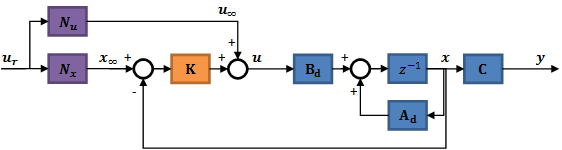


Where  is the value of the state vector and
  is the actuating signal value in steady-state. The feed-forward containing
  is crucial, because without it, the actuating signal is not in steady-state. (Basically it replaces an integrator.) The
  component calculates the goal values of the state variables according to the goal values of the output; hence it ensures that the input of
  is the error signal. It is worthy to note, that in case we use feed-forward alone (without the feedback) the system would eventually reach the end position as well; however not the way we planned.
So the goal is:
|
|
(6.13) |

For this:
|
|
(6.14) |


Determination of  :
:
|
|
(6.15) |

Calculation of  :
:
|
|
(6.16) |
Summarizing:
|
|
(6.17) |
Where  is a n x m nullmatrix and
  is a m x m identity matrix.
6.6.3. Design of the state observer
In real life situations we usually do not have the opportunity to measure all the state variables. It has several reasons; e.g. technically it is not possible to measure the given state variable or it cannot be measured accurately enough, the measurement is not cost efficient or the physical meaning of the state variable is unknown (e.g. in case of artificially created, identification based state space models). In such cases we need a state observer; the general function of the state observer is to determine the state of the system using the input and output signals, which can be easily measured in most cases. Therefore the state observer has two inputs: the block input ( ) and output (
 ); the output of the state observer is the vector of the observed state variables (
 ).
).
A state observer can only be applied, if the system is observable. Formally, a system is said to be observable if, knowing the inputs and outputs of the system in finite time, the system’s initial state can be determined. In case of time invariant systems in Discrete time it is true when the rank of the system’s observability matrix is maximal, that is its rank is n:
|
|
(6.18) |
The state observer in Discrete time :
|
|
(6.19) |
The estimation error:
|
|
(6.20) |
The goal is to keep the estimation error converging to zero ( ). Let us substitute the estimation error into the state observer equation and express it:
|
|
(6.21) |

Since:
|
|
(6.22) |

Therefore:
|
|
(6.23) |

It follows that:
|
|
(6.24) |

The last two term is always zero, if:
|
|
(6.25) |
Furthermore our goal is to get  as fast as possible. This is valid when the system is stable and fast:
|
|
(6.26) |
It can be ensured by proper selection of  . To have this we substitute
  and
and  in the equation of the estimation error:
|
|
(6.27) |
We transpose the equation:
|
|
(6.28) |
Let us compare this with the state feedback equation:
|
|
(6.29) |
It is visible, that the two equations are very similar and we can use that to determine the value of  , using the methods applied in case of state feedback. Consider the following system:
|
|
(6.30) |


If we design a state feedback for this system, the value of  is:
is:
|
|
(6.31) |

The only important remaining issue is the pole placement. To decide this matter we should use the greatest absolute valued pole in continuous time (obtained in the primary state feedback design) and choose many orders of magnitude larger. Selecting it carefully plays a crucial role in the stability of the system, especially if the actual system is different from the model, because the slow observer causes an unstable system. Therefore it is a basic requirement for a state observer that it must operate faster than the observed system. With this we get the following controller:


6.6.4. Integral control
Up to this point the designed controller works great theoretically: we decide the pole placement of the system, we determine how and how fast the system should reach steady state; and there is no steady-state error. What if the block is different from the one we used during design? In this case the state feedback will not place the poles to their designed location, since they are not in the place where we expect them to be; this may even lead to an unstable system and certainly lead to steady-state error, because the reference signal correction is based on the state space equations. On top of that, the state observer would not observe the real states.
The solution for the steady-state error is placing an integrator into the system. Using this we can eliminate the  part of the reference signal correction, since the integrator also has an output in case there is no error. In order to build in the integrator, introducing a new state variable is necessary:
|
|
(6.32) |

Here the Discrete time integrator is based on the left hand endpoint method. Extending the block state space equations with this:
|
|
(6.33) |
The state feedback have the following form:
|
|
(6.34) |
Thus in this case we design the state feedback to this extended system and we use the obtained  and
and  matrices as follows:


As we can see, the feed-forward containing  is replaced with the integrator, since the integrator ensures the lack of steady-state error. Placing the integrator in the feed-forward does not affect the design of the reference signal correction and the state observer.
6.6.5. Identification of the system
First we need to determine the model of the controller before the designing process can begin. To do that, we use the MATLAB System Identification Toolbox. The toolbox gives the possibility to identify systems from measurement results, which can be used for controller design. An important condition for this is to have a measurement which represents the system properly; since the program creates the system using the input and output values, any special phenomenon that does not occur in the measurement (but in the real system) is likely to not occur in the model as well. Before we start the measurement, it is practical to select the model we would use. In this case designing the controller would require a state space model in Discrete time . This can be easily derived from a transfer function. MATLAB offers several options to do that, we are going to use the ARMAX model. ARMAX is an acronym; it stands for AutoRegressive Moving-Average model with eXogenous inputs. A question regarding the emphasis of exogenous input may occur; hence before presenting the ARMAX model, we should understand two of its components, the AR and MA models. The AutoRegressive (AR) model:
|
|
(6.35) |
Where:
-

is the output value at
 time step
 -

is the internal input, white noise value at
 time step
 -
As we can see, this is a stochastic process. The Moving-Average (MA) has the same structure:
|
|
(6.36) |
Where . Since these models have no exogenous inputs, they are not suitable for describing the engine; however putting the models together and extending it with exogenous inputs we obtain the so called ARMAX model, which is eligible. The formula of the ARMAX model:
|
|
(6.37) |

Where:
-

is the exogenous input
-

is the system delay
-
, here the first coefficient is not 1. The reason for this is to have an arbitrary amplification of the system.
The purpose of the  term containing the white noise input is to map the measurement error. Actually this is the error of the equation:
|
|
(6.38) |
If there is no measurement error, then  :
:
|
|
(6.39) |
Therefore the transfer function:
|
|
(6.40) |
MATLAB can construct the transfer function for us, however understanding the basic operational principles may be useful. Substituting the values as parameters into the ARMAX equation, the magnitude of the error is given as a function of the polynomials coefficient. The value of the polynomials and thus the transfer function can be determined by minimizing the square of the error. The MATLAB does not determine the value of the delay time; it has to be given by the user.
From the transfer function we can develop a state space model in more than one way, e.g. observable canonical form, controllable canonical form, etc. In this methods, the physical meaning of the state variables are unknown; however this is not a disadvantage, since we do not expect this behaviour because of identification. In most cases the state space representation can be derived from the transfer function as follows:
|
|
(6.41) |
Let:
|
|
(6.42) |
With this:
|
|
(6.43) |


Consider the state variables as follows:
|
|
(6.44) |


Hence:
|
|
(6.45) |


The state space model:
|
|
(6.46) |
In possession of the state space model, the controller design may be performed.
6.6.6. Design of the control
After the review of the theoretical basics the design of the control can be done in the following three steps:
Identification of the system
-
Design and simulation of the control
-
Implementation and analysis of the control
These will be introduced in this section.
6.6.7. Identification of the motor
6.6.7.1. Analysis of the characteristics
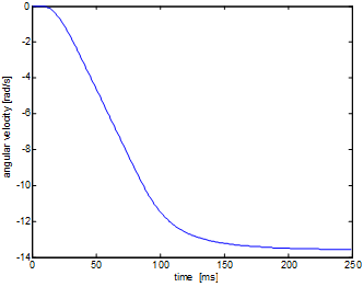
First the system had to be analysed. The DC motor available via the internet. With the help of the working system, the control of the input signals can be written in C programming language. By sending the C code to the remote monitoring station, it will be compiled and the result will be sent back. In this case the input of the motor is the required moment. From this moment, the current controller computes the output voltage. Thus the damaging input signals are prohibited. While the controlled output is the velocity of the motor. The maximal achievable angular velocity in the case of constant input signal (100 mNm):
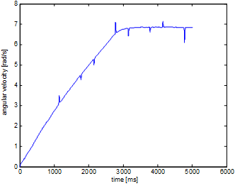
It can be noticed that the velocity is computed from the position by numerical differentiation and filtering. Therefore some pike still remain in the result. The designing of the filter will be detailed in later section.
In the case of 3 mNm :
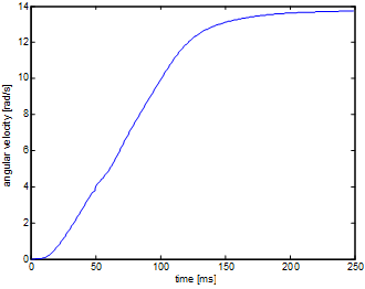
After more measurement, it can be stated that the maximum of the angular valocity is 14 rad/s. Furthermore it can be seen that the system gives higher response in the case of less moment. This means that the current control works wrong in the case of high input moments.
In the case of inversed direction of rotation (-3 mNm):
It can be seen that the absolute value of the extremes are about the same as in the previous case. In the next step, the system will be analysed by a quasi-static measurement to obtain the relation between the input moment and the output velocity. The measurement begin with a -3 mNm as an input and it increased slowly until +3 mNm:
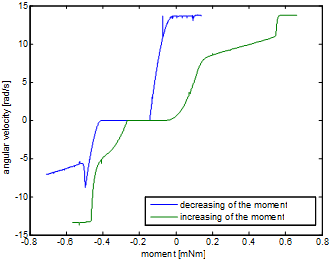
The figure above shows that the characteristic of the system is far away from linear:
-
Deadband: because of static friction.
-
There are more breakpoint.
-
Hysteresis: The direction of the moment change is also an important factor.
6.6.7.2. Design of the excitation for the identification
To achieve a well working control, the system has to be as linear as possible. Even the case of non linear system, every system can be linearized around a given working point. Thus, to demonstrate the operating of the control, a precision velocity controller will be made. At first the system is taken into the close area of the working point then the system pass to the precision control.
After the system is taken into the close area of the working point, a square wave signal is applied as input. The response of the system will be the basics of the identification. Then the picked linear section should be the linear section between 0.2mNm and 0.5mNm. For the identification of this, a square wave signal is used by setting of 4s as the time of period, 0.35mNm as the mid-torque and 0.15 as the amplitude. And 2 seconds was given to reach the working point:
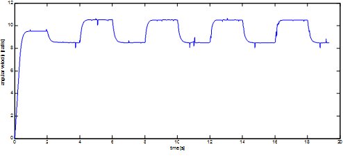
The 6-15.figure shows the output of the system. And this output well approximates the output of a linear system. The C code of the measurement is:
typedef struct
{
float Position;
float Velocity;
float Torque;
float StateVariable_5;
float StateVariable_6;
float StateVariable_7;
float StateVariable_8;
float StateVariable_9;
float StateVariable_10;
NewControllerData
NewControllerData CalculateController(
const float CurrentPosition,
const float OldPosition,
const float OldVelocity,
const float CurrentTime,
const float OldTime,
const float Old_StateVariable_5,
const float Old_StateVariable_6,
const float Old_StateVariable_7,
const float Old_StateVariable_8,
const float Old_StateVariable_9,
const float Old_StateVariable_10
NewControllerData ResultData; // result
//Filter coefficient
static float filB0 = 0, filB1 = 0.00013337, filB2 = 0.0012028, filB3 = 0.0009847099, filB4 = 7.3193E-05;
static float filA0 = 1, filA1 = -3.1152, filA2 = 3.6392, filA3 = -1.8895, filA4 = 0.36788;
//input
static float input0 = 0, input1 = 0, input2 = 0, input3 = 0, input4 = 0;
//filtered value
static float filter0 = 0, filter1 = 0, filter2 = 0, filter3 = 0, filter4 = 0;
float u;
//mid-value of the moment
float bias = 0.35;
//waiting for the set up
int start = 2000;
//time of the period
int period = 4000;
//amplitude
float amplitude = 0.15;
// Position is saved automatically
ResultData.Position = CurrentPosition;
// angular velocity is saved automatically
if (CurrentTime != 0.0f){
ResultData.Velocity = (1000.0f * (float)(CurrentPosition - OldPosition)/(float)(CurrentTime - OldTime));
}
else {
ResultData.Velocity = 0.0f;
}
//velocity filtering
input0 = ResultData.Velocity;
filter0 = (filB0 * input0 + filB1 * input1 + filB2 * input2 + filB3 * input3 + filB4 * input4 - (filA1 * filter1 + filA2 * filter2 + filA3 * filter3 + filA4 * filter4)) / filA0;
input4 = input3; input3 = input2; input2 = input1; input1 = input0;
filter4 = filter3; filter3 = filter2; filter2 = filter1; filter1 = filter0;
ResultData.StateVariable_5 = filter0;
//the moment
if(CurrentTime < start)
{
u = 0;
}
else
{
u = (((int)CurrentTime - start) % period - period / 2 > 0 ? amplitude : -amplitude);
}
ResultData.Torque = u + bias;
ResultData.StateVariable_6 = u;
return ResultData;
}
6.6.7.3. Identification with the help of the MATLAB
First the results of the measurement have to be uploaded into the MATLAB. Then the transient phase should be cut off, it’s won’t be needed. Instead of the true velocity and moment, the their deviations from the working point is used for the identification of the system. Furthermore the sampling time is 1ms. By performing the previous steps, the iddata command can generate the neccessary data structure for the System Identification Toolbox. Thereafter the degrees of the polynomials should be specified for the ARMAX model ( is the degree of the
  ,
,  is the degree of the
  ,
,  is the degree of the
  ,
,  is the deadband). Then
  row vector can be composed, where
  and
and  . The higher values of the degree of the polynomial results in higher uncertainty of the identification, in which case the MATLAB shows the „Warning: Pole locations are more than 10% in error.” message. This is important because the pole locations has to be changed, and the method doesn’t work well if the poles aren’t in the right position. Fortunately the identification takes only a few seconds, so many types of the setting should be tried. The identification can be run with the help of armax command. The result of this command will be the data structure of the system, whereof the th2poly function compute the descriptive row vectors of the polinoms. In these, the coefficients are ordered according to descending exponent values of the
  terms, so the
  is the last term. Of course, there should be zero coefficients as well. Actually in the this step the numerator and the denominator of the discrete transfer function are obtained, thus the tf can compute the discreteized form of the transfer function. The MATLAB code of the identification is:
start=1800;                                 %point of begin
y=velocity2(start:end)-velocity2(start);    %measurement vector of the angular velocity
u=torque2(start:end)-torque2(start);        %vector of the moment
n=3;                                        %number of the states
Ts=0.001;                                   %sampling time
z=iddata(y,u,Ts);                           %upload of the measured data
nn=[n,1,1,1];                               %set the degrees of the polynoms
tharmax=armax(z,nn);                        %identification
[A,B,C]=th2poly(tharmax);                   %read of the polys
sys=tf(B,A,Ts);                             %transfer function
The transfer function is:
|
|
(6.47) |
It is hard to see that this result is good or not. Therefore the response of the identified system should be computed by applying the input of the real system:
yid=idsim(tharmax,u,zeros(n,1)); %response of the identified system
t=0:Ts:(size(y)-1)*Ts; %time vector
figure(1); %new figure
plot(t,y,t,yid); %plot
legend('mesured','identified'); %legend
xlabel('time [s]'); %horizontal
ylabel('angular velocity [rad/s]'); %vertical
The operation of the identified system can be checked with the help of idsim function which calculate the output vector with respect of the input vector and initial states. Then the plot of the results is:
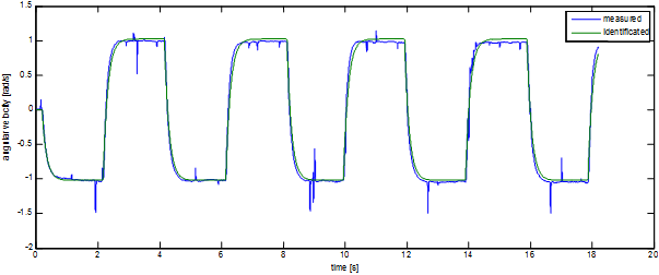
It can be seen in the figure that the model well approximate the experience. It has to be mentioned that the used excitation for the identification is can be optional, but it has to be suitable to specify the system features. So the result of the identification algorithm describe the real system well and with high degree of certainty in the case of the given exciting.
To design the control, it is necessary to know the discretized form of the state space model of the system, what can be obtained with the help of ss command:
sysd=ss(sys);                               %state space model
[Phi Gamma C D]=ssdata(sysd);               %read the matrices
Now everything ready for the design of the control.
6.6.8. Design of the control
6.6.8.1. Control without of the integrator
First the parameter of the required system has to be defined, then the pole of the continous time system also has to be defined. The response of the reqiured system is:
a=2;                                        %percentage of the set up
Tap=0.2;                                    %time of control
xi=0.8;                                     %dumping
w0=log(100/a)/Tap/xi;                       %natural frequency

sdom1=-w0*xi+1i*w0*sqrt(1-xi^2);            %dominant pole
sdom2=conj(sdom1);
scinf=-4*w0;                                %auxiliary pole to control
soinf=scinf*5;                              %auxiliary pole to observe
if(-soinf>0.5/Ts)                           %Shannon-theory check
    display('Sampling time is too short!');
end;

%model of the required system
tcsys=zpk([],[sdom1, sdom2, scinf*ones(1,n-2)],-w0^2*scinf^(n-2));
figure(2);                                  %new plot
step(tcsys);                                %step response
The response of the step function is:
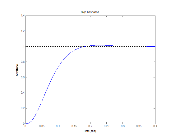
Then the poles in discretized time is:
%calculation of the poles for discrete time
zdom1=exp(sdom1*Ts);
zdom2=exp(sdom2*Ts);
zcinf=exp(scinf*Ts);
zoinf=exp(soinf*Ts);
Then the state feedback, the reference signal correction and state observation are can be done according to the theoretical introduction:
%checking of controllability
Mc=ctrb(Phi,Gamma);
if rank(Mc)~=n
disp('The system can not be controlled!');
end
%design of the state feedback
phic=[zdom1 zdom2 zcinf*ones(1,n-2)]; %new poles
K=acker(Phi,Gamma,phic); %pole placement
%calculation of the base-signal correction
NxNu=inv([Phi-eye(n) Gamma;C 0])*[zeros(n,1);1];
Nx=NxNu(1:n);
Nu=NxNu(n+1);
%checking of observability
Mo=obsv(Phi,C);
if rank(Mo)~=n
disp('The system can not be observed!');
end
%design of state observer
phio=ones(1,n)*zoinf; %poles of the observer
G=acker(Phi',Phi'*C',phio)'; %pole transfer on dual system
F=Phi-G*C*Phi;
H=Gamma-G*C*Gamma;
At this point the design of the control is finished. To check the control, it is recommended to done some simulation in the Simulink.
Build the following model:
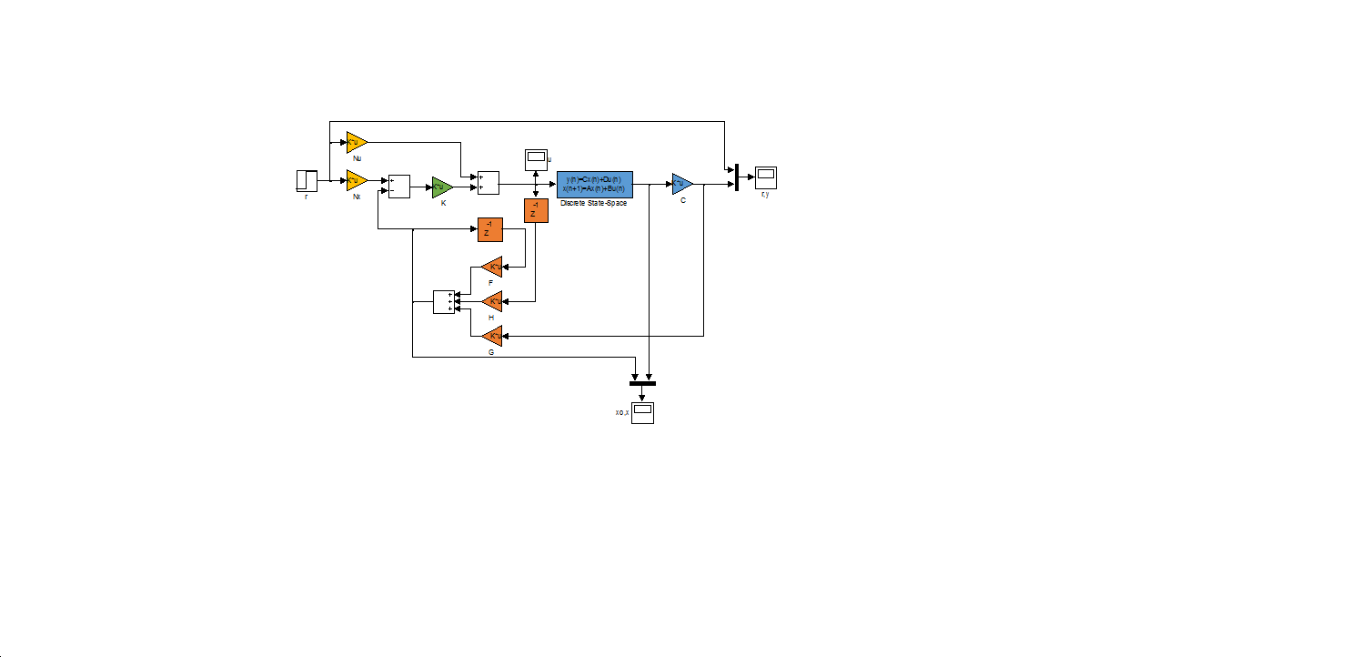
The section is divided to two parts. In the Discrete time state space model every states are taken out which useful to check the operation of the state estimator. While the signal which contains the C gain is the output. Take care of that the sampling time is given for every element! Thereafter the results are:
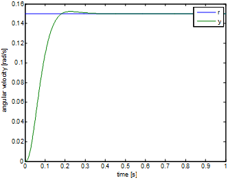
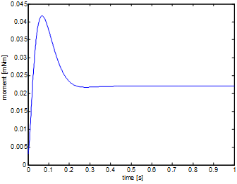
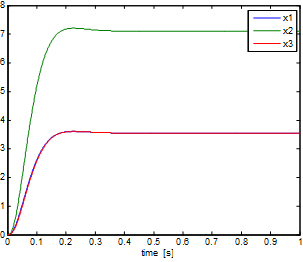
The control works well, the intervening signal doesn’t run over the linear section.
6.6.9. Integral control
For the design of the integral control, at first the equation of the state has to be expanded with the integrator:
iPhi=[Phi, zeros(n,1); Ts*C, 1];
iGamma=[Gamma; 0];
iC=[C 0];
To design the state feedback, one more pole is necessary:
siinf=scinf;                                %Pole for integrator
ziinf=exp(siinf*Ts);
if(-min([siinf soinf])>0.5/Ts)              %checking of Shannon-theory
    display('The sampling time is too short!');
end;
Then the state feedback control can be design:
iPhic=[zdom1 zdom2 zcinf*ones(1,n-2) ziinf];%new poles
iK=acker(iPhi,iGamma,iPhic);                %pole placement
K=iK(1:n);                                  %state feedback
Ki=iK(n+1);                                 %integrator feedback
The modified Simulink model is:
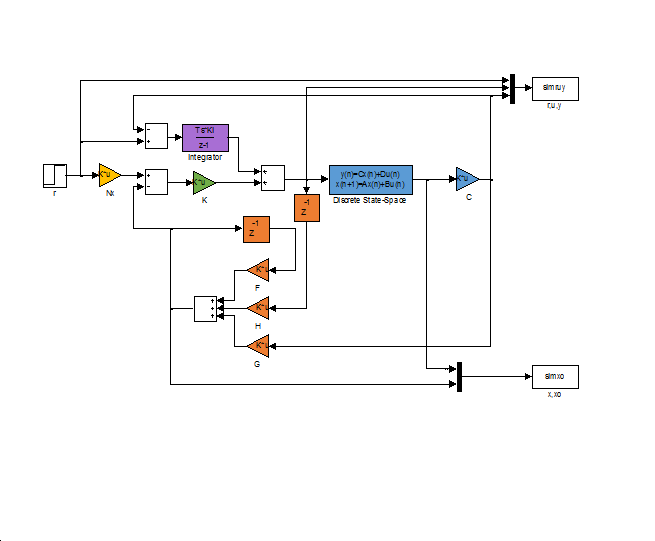
The results of the simulation are:
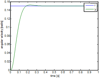
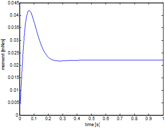
It can been seen that the response of the system doesn’t change. The difference will be noticeable if there were a 0.01mNm mistake in the calculation of the working point. In which case the response of the system without the integrator is:
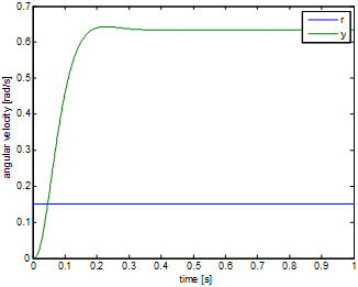
While the response of the system with the integrator is:
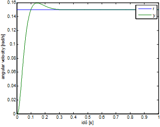
The figures above are clearly show that the response with the integrator is close to the ideal, while the control without the integrator is applicable only in the ideal case.
6.6.10. Filter design for velocity measurement
The angular velocity is computed from the position by numerical derivating. Therefore the input should be noisy. Thus this input has to be filtered. To design the filter, there are two controversial requirement: in the one hand the filter has to be as fast as possible because the delay caused by the filter reduce the stability of the system. On the other hand the noise has to be well filtered. The simplest filter can be achived by series connecting of the single capacity elements. Where -20dB/decade is the change of the amplification of the single capacity element. This type of the filter can be designed with the help of MATLAB. The continuous and discrete transfer functions can be calculated from value of the degree and locations of the poles:
filT=0.001;                                 %filter time constant
filN=3;                                     %filter degree

%continous time filter
filsys=tf(zpk([],-ones(1,filN)/filT,(1/filT)^filN));
dfilsys=c2d(filsys,Ts,'zoh');               %discrete time version
The implementation of the filter can be done after the discrete transfer function is obtained, but first analyse the operation of the filter (Bode diagram, step response and noisy input response):
figure(1);
dbode(dfilsys.num{1},dfilsys.den{1},Ts)     %Bode diagram

figure(2);
step(dfilsys);                              %step response

figure(3);
v=velocity(start:end)-velocity(start);      %noisy signal
lsim(dfilsys,v,t);                          %filtering of noisy signal
The results are:
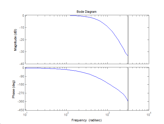
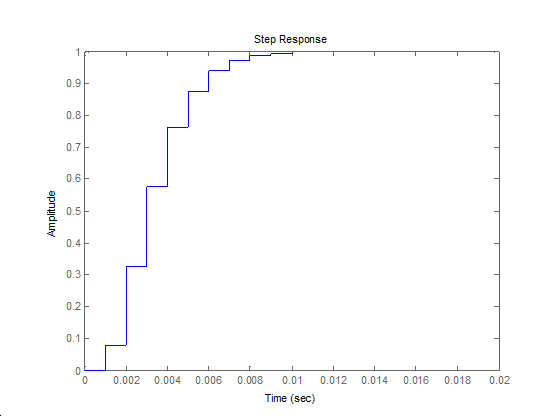
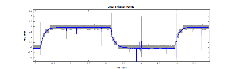
6.6.11. Implementation
The integration of the control can be written in C language. Although the online test environment has some limit. There aren’t possible to use arrays, it is impossible to define own functions or global variables. Therefore it is well recommended to create a program which translate the MATLAB code into C code. This program is introduced in the appendix.
6.6.12. Control without integrator
C code
#include <windows.h>
#include <stdio.h>
#include <rtapi.h>
#include <math.h>
#include <string.h>
#define PI 3.14159265358979323846
typedef struct
{
float Position;
float Velocity;
float Torque;
float StateVariable_5;
float StateVariable_6;
float StateVariable_7;
float StateVariable_8;
float StateVariable_9;
float StateVariable_10;
} NewControllerData;
NewControllerData CalculateController(
const float CurrentPosition,
const float OldPosition,
const float OldVelocity,
const float CurrentTime,
const float OldTime,
const float Old_StateVariable_5,
const float Old_StateVariable_6,
const float Old_StateVariable_7,
const float Old_StateVariable_8,
const float Old_StateVariable_9,
const float Old_StateVariable_10
)
{
NewControllerData ResultData; // result
static float filB0 = 0, filB1 = 0.080301, filB2 = 0.1544, filB3 = 0.017881;
static float filA0 = 1, filA1 = -1.1036, filA2 = 0.40601, filA3 = -0.049787;
static float input0 = 0, input1 = 0, input2 = 0, input3 = 0;
static float filter0 = 0, filter1 = 0, filter2 = 0, filter3 = 0;
static float Nu0_0 = 0.14662;
static float Nx0_0 = 23.677, Nx1_0 = 47.353, Nx2_0 = 23.677;
static float K0_0 = -1.2522, K0_1 = 0.81068, K0_2 = -0.37451;
static float F0_0 = 2.7896, F0_1 = -1.889, F0_2 = 0.84863, F1_0 = 2, F1_1 = -0.94991, F1_2 = 0, F2_0 = 0, F2_1 = 0.13587, F2_2 = 0;
static float G0_0 = 26.977, G1_0 = 44.981, G2_0 = 17.242;
static float H0_0 = 0.0625, H1_0 = 0, H2_0 = 0;
static float Gamma0_0 = 0.0625, Gamma1_0 = 0, Gamma2_0 = 0;
static float Phi0_0 = 2.7896, Phi0_1 = -1.3193, Phi0_2 = 0.84863, Phi1_0 = 2, Phi1_1 = 0, Phi1_2 = 0, Phi2_0 = 0, Phi2_1 = 0.5, Phi2_2 = 0;
static float C0_0 = 0, C0_1 = 0, C0_2 = 0.042236;
static float r = 0;
static float xu = 0;
static float xuL = 0;
static float xk0 = 0, xk1 = 0, xk2 = 0;
static float xkL0 = 0, xkL1 = 0, xkL2 = 0;
static float y = 0;
// Position is saved automatically
ResultData.Position = CurrentPosition;
// Angular velocity is saved automatically
if (CurrentTime != 0.0f){
ResultData.Velocity = (1000.0f * (float)(CurrentPosition - OldPosition)/(float)(CurrentTime - OldTime));
}
else {
ResultData.Velocity = 0.0f;
}

r=sin(CurrentTime/1000)/2-1;
input0 = ResultData.Velocity;
filter0 = (filB0 * input0 + filB1 * input1 + filB2 * input2 + filB3 * input3 - (filA1 * filter1 + filA2 * filter2 + filA3 * filter3)) / filA0;
input3 = input2; input2 = input1; input1 = input0;
filter3 = filter2; filter2 = filter1; filter1 = filter0;
if(CurrentTime < 2000) ResultData.Torque =   3.5000e-001;
else
{
y = filter0 +   -9.5218e+000;
xk0 = F0_0 * xkL0 + F0_1 * xkL1 + F0_2 * xkL2 + H0_0 * xuL + G0_0 * y;
xk1 = F1_0 * xkL0 + F1_1 * xkL1 + F1_2 * xkL2 + H1_0 * xuL + G1_0 * y;
xk2 = F2_0 * xkL0 + F2_1 * xkL1 + F2_2 * xkL2 + H2_0 * xuL + G2_0 * y;
xu = Nu0_0 * r + K0_0 * (Nx0_0 * r - xk0) + K0_1 * (Nx1_0 * r - xk1) + K0_2 * (Nx2_0 * r - xk2);
if(xu > 1) xu = 1;
if(xu < -1) xu = -1;
ResultData.Torque = xu +   3.5000e-001;
xuL = xu;
xkL0 = xk0;
xkL1 = xk1;
xkL2 = xk2;
}
ResultData.StateVariable_5 = r;
ResultData.StateVariable_6 = y;
return ResultData;
}
6.6.13. Results of the measurement

As the figure show the control well approximate the reference signal in spite of the facts there are no integrator in the control loop and modelled system is different from the real one. And of course the bigger deviation from the working point cause bigger error between the output and the reference signals.
6.6.14. Control with the integrator
C code
#include <windows.h>
#include <stdio.h>
#include <rtapi.h>
#include <math.h>
#include <string.h>
#define PI 3.14159265358979323846
typedef struct
{
float Position;
float Velocity;
float Torque;
float StateVariable_5;
float StateVariable_6;
float StateVariable_7;
float StateVariable_8;
float StateVariable_9;
float StateVariable_10;
} NewControllerData;
NewControllerData CalculateController(
const float CurrentPosition,
const float OldPosition,
const float OldVelocity,
const float CurrentTime,
const float OldTime,
const float Old_StateVariable_5,
const float Old_StateVariable_6,
const float Old_StateVariable_7,
const float Old_StateVariable_8,
const float Old_StateVariable_9,
const float Old_StateVariable_10
)
{
NewControllerData ResultData; // result
static float filB0 = 0, filB1 = 0.080301, filB2 = 0.1544, filB3 = 0.017881;
static float filA0 = 1, filA1 = -1.1036, filA2 = 0.40601, filA3 = -0.049787;
static float input0 = 0, input1 = 0, input2 = 0, input3 = 0;
static float filter0 = 0, filter1 = 0, filter2 = 0, filter3 = 0;
static float Nu0_0 = 0.14662;
static float Nx0_0 = 23.677, Nx1_0 = 47.353, Nx2_0 = 23.677;
static float K0_0 = 0.2386, K0_1 = -0.5816, K0_2 = 0.9255, K0_3 = 1.9278;
static float F0_0 = 2.7896, F0_1 = -1.889, F0_2 = 0.84863, F1_0 = 2, F1_1 = -0.94991, F1_2 = 0, F2_0 = 0, F2_1 = 0.13587, F2_2 = 0;
static float G0_0 = 26.977, G1_0 = 44.981, G2_0 = 17.242;
static float H0_0 = 0.0625, H1_0 = 0, H2_0 = 0;
static float Gamma0_0 = 0.0625, Gamma1_0 = 0, Gamma2_0 = 0;
static float Phi0_0 = 2.7896, Phi0_1 = -1.3193, Phi0_2 = 0.84863, Phi1_0 = 2, Phi1_1 = 0, Phi1_2 = 0, Phi2_0 = 0, Phi2_1 = 0.5, Phi2_2 = 0;
static float C0_0 = 0, C0_1 = 0, C0_2 = 0.042236;
static float r = 0;
static float xu = 0;
static float xuL = 0;
static float xk0 = 0, xk1 = 0, xk2 = 0;
static float xkL0 = 0, xkL1 = 0, xkL2 = 0;
static float y = 0;
static float i = 0;
// Position is saved automatically
ResultData.Position = CurrentPosition;
// Angular velocity is saved automatically
if (CurrentTime != 0.0f){
ResultData.Velocity = (1000.0f * (float)(CurrentPosition - OldPosition)/(float)(CurrentTime - OldTime));
}
else {
ResultData.Velocity = 0.0f;
}

r=sin(CurrentTime/1000)/2-1;
input0 = ResultData.Velocity;
filter0 = (filB0 * input0 + filB1 * input1 + filB2 * input2 + filB3 * input3 - (filA1 * filter1 + filA2 * filter2 + filA3 * filter3)) / filA0;
input3 = input2; input2 = input1; input1 = input0;
filter3 = filter2; filter2 = filter1; filter1 = filter0;
if(CurrentTime < 2000) ResultData.Torque =   3.5000e-001;
else {
y = filter0 +   -9.5218e+000;
xk0 = F0_0 * xkL0 + F0_1 * xkL1 + F0_2 * xkL2 + H0_0 * xuL + G0_0 * y;
xk1 = F1_0 * xkL0 + F1_1 * xkL1 + F1_2 * xkL2 + H1_0 * xuL + G1_0 * y;
xk2 = F2_0 * xkL0 + F2_1 * xkL1 + F2_2 * xkL2 + H2_0 * xuL + G2_0 * y;
i += 0.0019278 * (r - y);
xu = i + K0_0 * (Nx0_0 * r - xk0) + K0_1 * (Nx1_0 * r - xk1) + K0_2 * (Nx2_0 * r - xk2);
if(xu > 1) xu = 1;
if(xu < -1) xu = -1;
ResultData.Torque = xu +   3.5000e-001;
xuL = xu;
xkL0 = xk0;
xkL1 = xk1;
xkL2 = xk2;
}
ResultData.StateVariable_5 = r;
ResultData.StateVariable_6 = y;
return ResultData;
}
6.6.15. Results of the measurement in the case of integrator
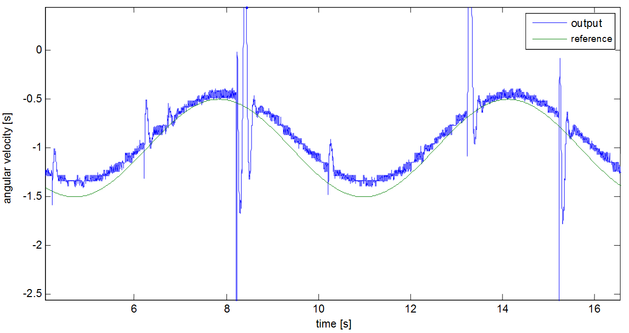
The control with the integrator works well and the error between the reference and output signal is neglactable.
6.6.16. Appendix
The complete MATLAB code of the control
%%settings
integrator=true;
idplots=true;
stateplots=true;
outplots=true;
filterdesign=true;
%% Identification
start=1800;                                 %start time
y=velocity2(start:end)-velocity2(start);    %vector of the measured angular velocity
u=torque2(start:end)-torque2(start);        %vector of the measured torque

n=3;                                        %number of state variables
Ts=0.001;                                   %sampling time
z=iddata(y,u,Ts);                           %measured data
nn=[n,1,1,1];                               %determination of degree numbers
tharmax=armax(z,nn);                        %identification
[A,B,C]=th2poly(tharmax);                   %polynomials read
sys=tf(B,A,Ts);                             %transfer function

yid=idsim(tharmax,u,zeros(n,1));            %response of the identified system
t=0:Ts:(size(y)-1)*Ts;                      %time vector
if(idplots)
figure(1);                                  %new diagram
plot(t,y,t,yid);                            %diagram
legend('measured','identified');            %legend
xlabel('time [s]');                         %x axis
ylabel('angular velocity [rad/s]'           %y axis
end;
sys

%%design of filter
if(filterdesign)
filT=0.001;                                 %filter time constant
filN=3;                                     %filter degree

%continous  time filter
filsys=tf(zpk([],-ones(1,filN)/filT,(1/filT)^filN));
dfilsys=c2d(filsys,Ts,'zoh');               %discrete time version

figure(1);
dbode(dfilsys.num{1},dfilsys.den{1},Ts)     %Bode diagram

figure(2);
step(dfilsys);                              %step response

figure(3);
v=velocity(start:end)-velocity(start);      %noisy signal
lsim(dfilsys,v,t);                          %filtering of the noisy signal
end;
%%design of controller
sysd=ss(sys);                               %model of state space
[Phi Gamma C D]=ssdata(sysd);               %read matrixes

a=2;                                        %what percent we stand
Tap=0.2;                                    %control time
xi=0.8;                                     %mitigation
w0=log(100/a)/Tap/xi;                       %own frequency

sdom1=-w0*xi+1i*w0*sqrt(1-xi^2);            %dominant poles
sdom2=conj(sdom1);
scinf=-4*w0;                                %auxiliary poles for the controller
soinf=scinf*5;                              %auxiliary poles for the observer
siinf=scinf;                                %auxiliary poles for the integrator
%checking of Shannon-theory
if(-soinf>0.5/Ts || (integrator && -min([siinf soinf])>0.5/Ts))
    display('The  settling time is too short!');
end;

%model of the target system with unit grain
if(idplots)
tcsys=zpk([],[sdom1, sdom2, scinf*ones(1,n-2)],-w0^2*scinf^(n-2));
figure(2);                                  %new diagram
step(tcsys);                                %calculation of the step response
end;

%calculating of the poles for discrete time
zdom1=exp(sdom1*Ts);
zdom2=exp(sdom2*Ts);
zcinf=exp(scinf*Ts);
zoinf=exp(soinf*Ts);
ziinf=exp(siinf*Ts);

%checking of controllability
Mc=ctrb(Phi,Gamma);
if rank(Mc)~=n
   disp(‘The system is uncontrollable!');
end

%design of the state feedback
if(integrator)
iPhi=[Phi, zeros(n,1); Ts*C, 1];
iGamma=[Gamma; 0];
iC=[C 0];
iPhic=[zdom1 zdom2 zcinf*ones(1,n-2) ziinf];%new poles
iK=acker(iPhi,iGamma,iPhic);                %pole placement
K=iK(1:n);                                  %state feedback
Ki=iK(n+1);                                 %feedback of the integrator
else
phic=[zdom1 zdom2 zcinf*ones(1,n-2)];       %new poles
K=acker(Phi,Gamma,phic);                    %pole placement
end

%calculating of the base-signal correction
NxNu=inv([Phi-eye(n) Gamma;C 0])*[zeros(n,1);1];
Nx=NxNu(1:n);
Nu=NxNu(n+1);

%checking of observability
Mo=obsv(Phi,C);
if rank(Mo)~=n
   disp(‘The system can not be observed!');
end

%design of state observer
phio=ones(1,n)*zoinf;                       %poles of the observer
G=acker(Phi',Phi'*C',phio)';                %pole transfer on dual system
F=Phi-G*C*Phi;
H=Gamma-G*C*Gamma;


%% simulation
if(integrator)
    open('szabint');
    sim('szabint');
else
    open('szab');
    sim('szab');
end;
rout=simruy(:,1);
uout=simruy(:,2);
yout=simruy(:,3);
tout=[0; tout];

if(outplots)
figure(3);
plot(tout,rout,tout,yout);
xlabel('time [s]');
ylabel('angular velocity [rad/s]');
legend('r','y');

figure(4);
plot(tout,uout);
xlabel('time [s]');
ylabel('torque [mNm]');
end;

if(stateplots)
figure(5);
plot(tout,simxo(:,1:n));
xlabel('time [s]');
ylabel('');
legend('x1','x2','x3');

figure(6);
plot(tout,simxo(:,n+1:2*n));
xlabel('time [s]');
ylabel('');
legend('x1','x2','x3');
end;