Chapter 8. Sensorless Control with Speed Estimators
8.1. Sensorless FOC Techniquess
In the case of induction motors, field oriented control (FOC), as compared to other control strategies, has great advantages. However, FOC requires the measurement of the speed, which may be technically unrealisable or extremely expensive. As a consequence, there is a strong interest in the FOC without any speed sensors. During the last five years several sensorless schemes have been proposed in the professional literature to identify the rotor speed by voltage and current measurements only [20]. In general, there is a trade-off between control performance and the the simplicity of implementation. Consequently, it is not possible to select the “best” general sensorless scheme [21]. The main objective of this chapter is to give an overview of the most important methods used in sensorless control of AC drives, to analyse them, and to compare a few of them with the traditional speed sensor-based methods. Bearing in mind the huge implementation efforts in the field of such kinds of applications, this chapter will focus on the simulation of the methods. Let us now review the basic concepts of the available field oriented sensorless techniques. This summary is mainly based on [21] and [20].
-
Speed Estimators (SE).
-
Model Reference Adaptive Systems (MRAS).
-
Luenberger Speed Observers (LSO).
Speed estimators use measured stator currents and estimated or observed stator (or rotor) flux to estimate the speed. In most cases the rotor speed  is calculated as the difference between the synchronous pulsation
  and the slip pulsation
  :
:
|
|
(8.1) |
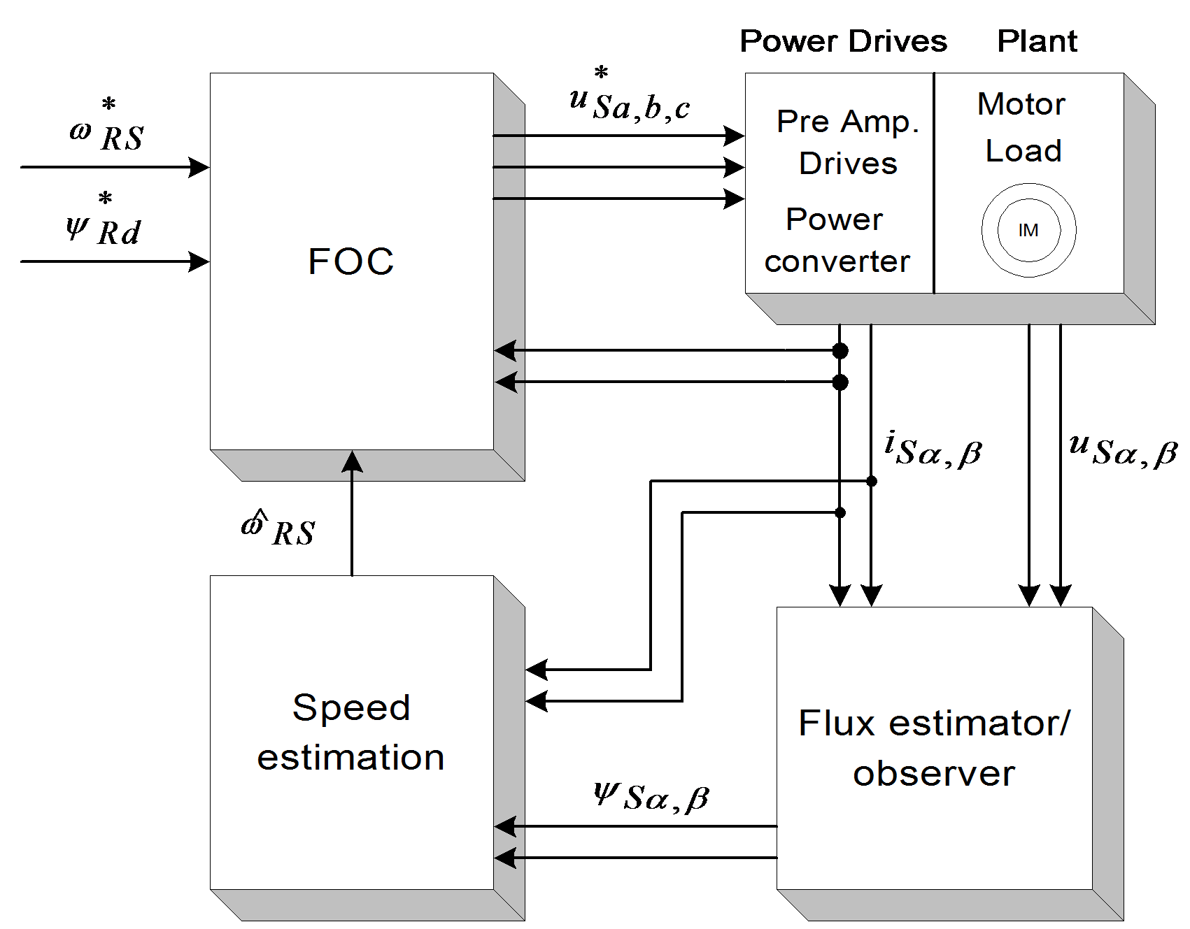
Notice that the derivative of the flux is present, which means that the input voltages directly influence the estimated speed. The general model of this technique is shown in Figure 81. No feedback exists in the controlling cycle.
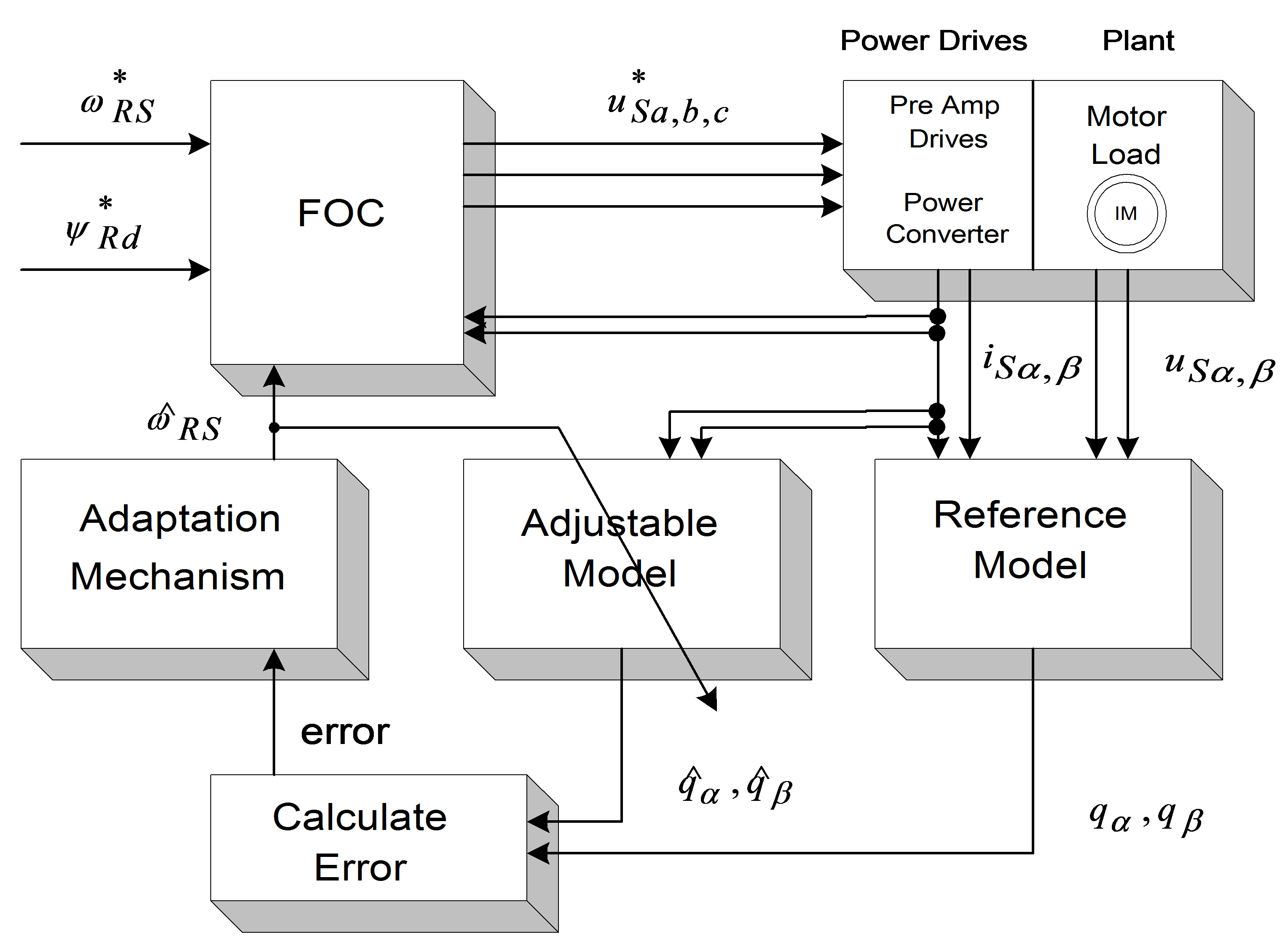
Model Reference Adaptive Systems are based on the comparison of the output of two estimators: one is the reference model, the other is the adjustable model. A suitable adaptation algorithm calculates the rotor speed from the output error. There is a feedback in the controlling cycle because the adjustable model uses the rotor speed. MRAS methods differ from each other in the output quantity q used for error calculation (see Figure 82.). The adaptation mechanism is the same for all model reference strategies:
|
|
(.8.2) |

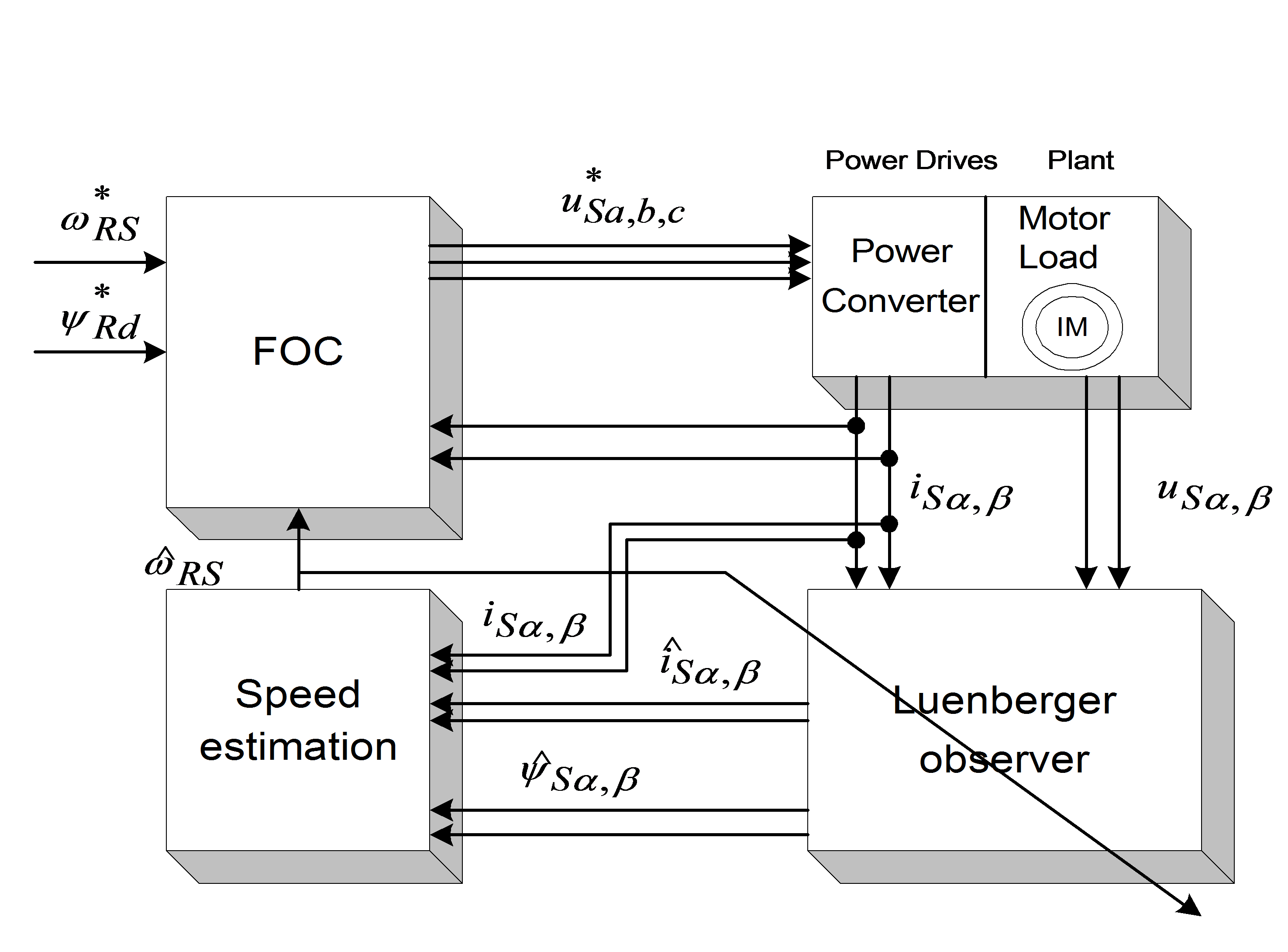
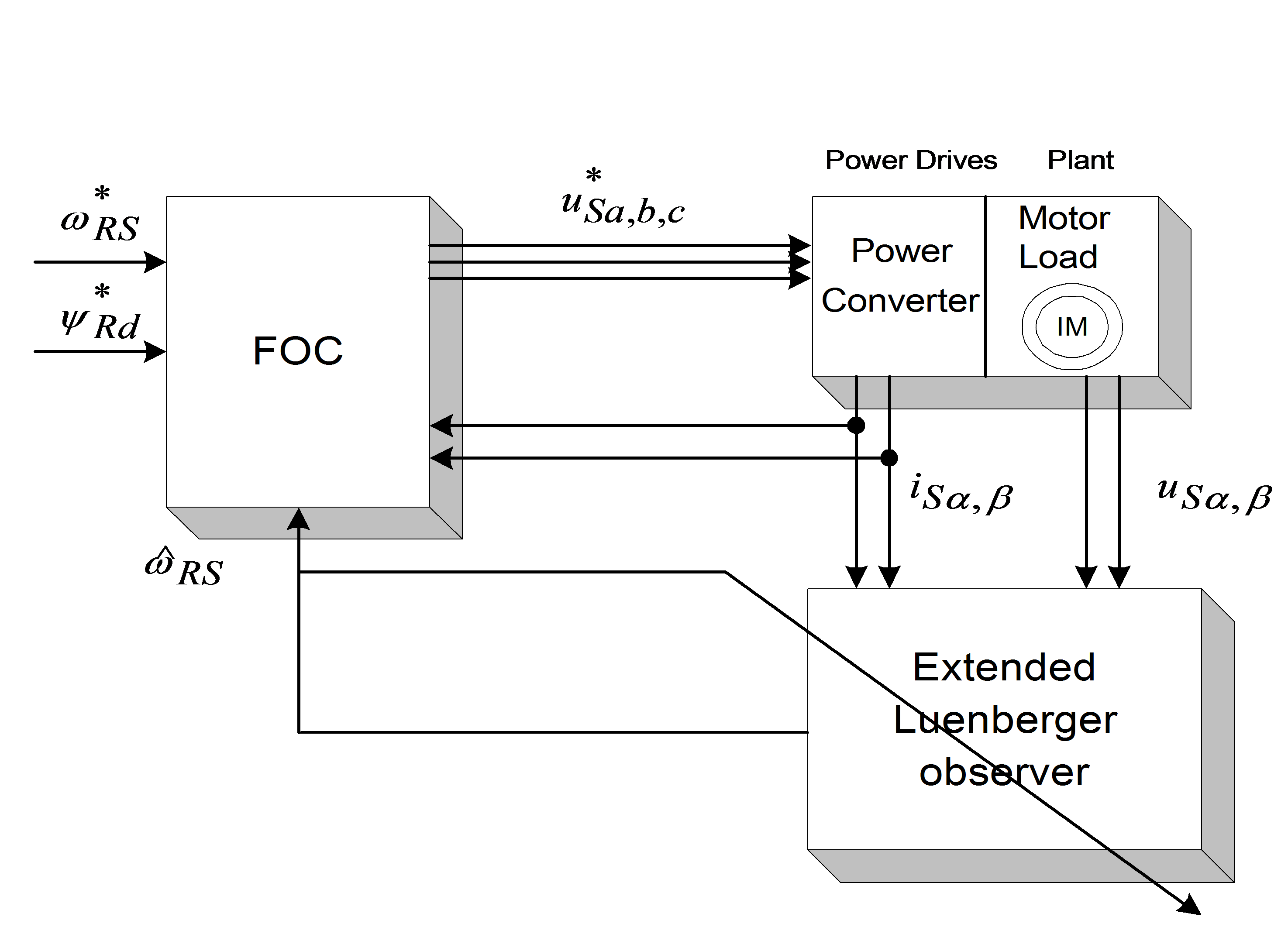
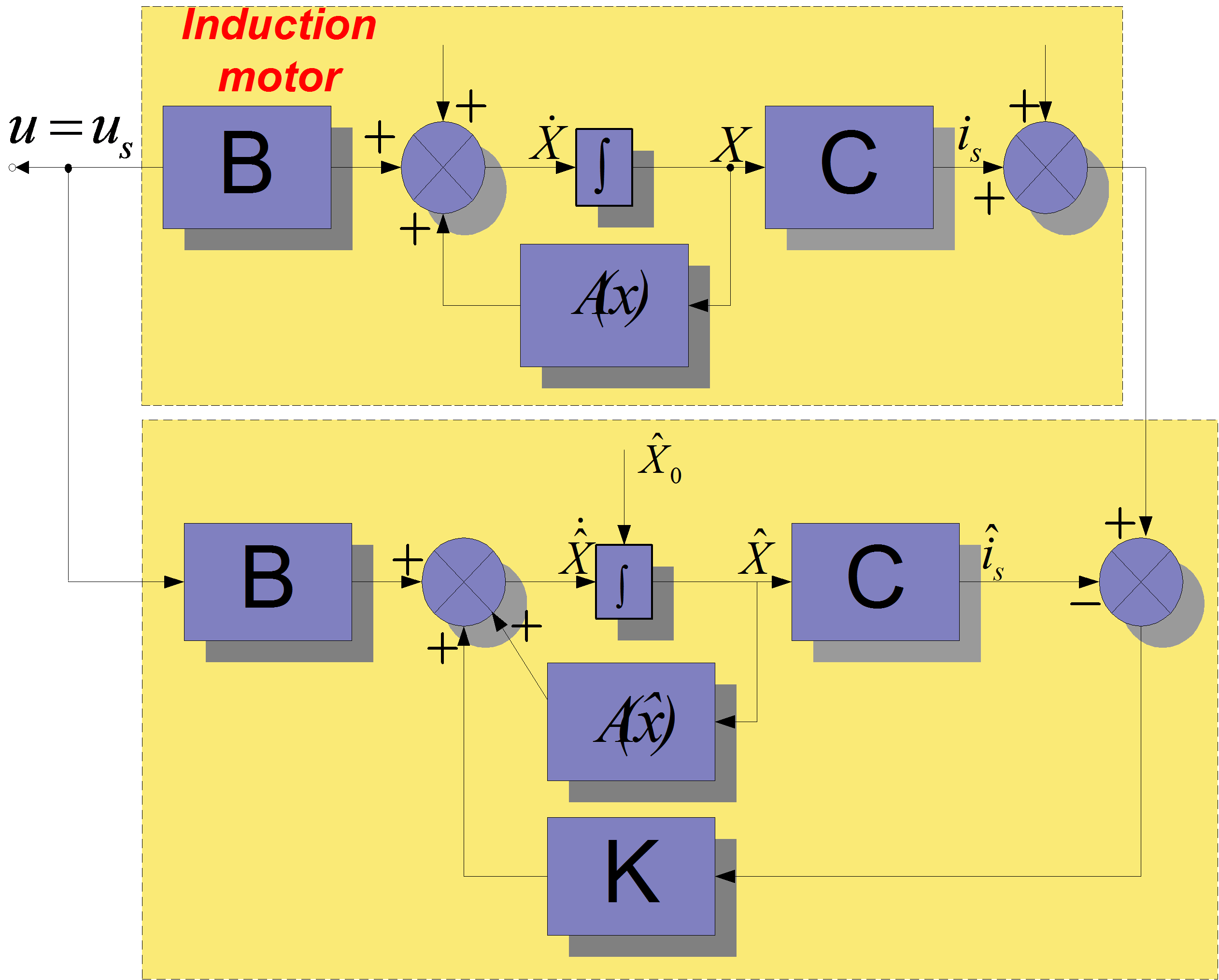
Luenberger Observer (LO) techniques are based on the fact that the rotor flux and the stator current are estimated by a deterministic (Luenberger) observer, and the rotor speed is calculated with an adaptive scheme using the stator current error and the estimated flux. If the rotor speed is included in the state variables of the observer, the scheme differs from the previous one. This is called the Extended Luenberger Observer (ELO). The two schemes are shown in Figure 8-3. and Figure 8-4. In terms of classification, these techniques are similar to the model reference adaptive methods if the motor is treated as the reference system, and the observer as the adjustable model.
The blockdiagram of the Kalman Filter based method is the same as that in the case of the Luenberger observer. The difference between them is the observer itself. The Kalman filter is a statistically optimum observer if the covariance matrices of the various noises are known. It means that the Kalman filter directly cares for the effects of the disturbance noises in- and outside the system. The errors in the parameters will also be handled as noise. A great difference in computation time exists between the Kalman filter and the Luenberger observer. In the case of the Kalman filter techniques, the observer gain matrix has to be computed in each controlling cycle. That is, many matrix operations and matrix inversions are required, resulting in a problem when implementing it in real-time. Generally speaking, the Kalman filter was developed for stochastic systems, and the Luenberger observer is, in fact, its deterministic case.
After reviewing the main ideas of the sensorless techniques, we would like to compare their performance, in order to select one of them for adaptation in the field oriented reference frame. In [21], this comparison is performed on the basis of the following set of criteria:
-
response time to load change steps,
-
low speed operation,
-
steady state error,
-
computation time,
-
parameter sensitivity,
-
noise sensitivity.
The problem for SE, MRAS, and KFT is that a trade-off exists between the good disturbance rejection and the short settling time when setting the speed PI gains. This problem does not occur in the case of LSO. SE, LSO, and KFT may work at very low speed (at e.g., at 20 rpm), while there is a minimum speed (about 100 rpm) for MRAS. SE and MRAS have a small steady state error when the motor is loaded [21]. KF algorithms contain many matrix operations, which causes problems when they are implemented on a DSP system. This problem does not exist at SE, MRAS and LO. When rotor resistance is detuned, LO seems to give the best result, and LE, MRAS, and KFT work similarly. The only stochastic system-based scheme, KFT gives an outstanding result when measurement and process noises are present. Our main specifications are to have a good dynamic behaviour at low frequencies, and a computational complexity as small as possible. EKF seems to give the best behaviour with respect to the criteria taken the most often into consideration, and is better in the case of measurement and process noises, however, it requires high processor capacity.
According to all these considerations, EKF has been selected for deeper analysis
8.2. Observers’ Basics
Let us first formulate the problem of observers. Let us take a system which has some internal states, these state variables are normally not measurable, so we usually measure only substitute variables. If we want to know these internal state variables for some reason, for example, we want to be able to control them, then we have to calculate them. It is not always possible to calculate these variables directly from the measured outputs. Let us consider a system with the following form, which is actually the so-called the ‘state space form’. (Note that all symbols that denote matrices or vectors are underlined).

 ,(8.3)
|
|
(,8.4) |

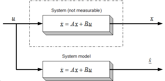
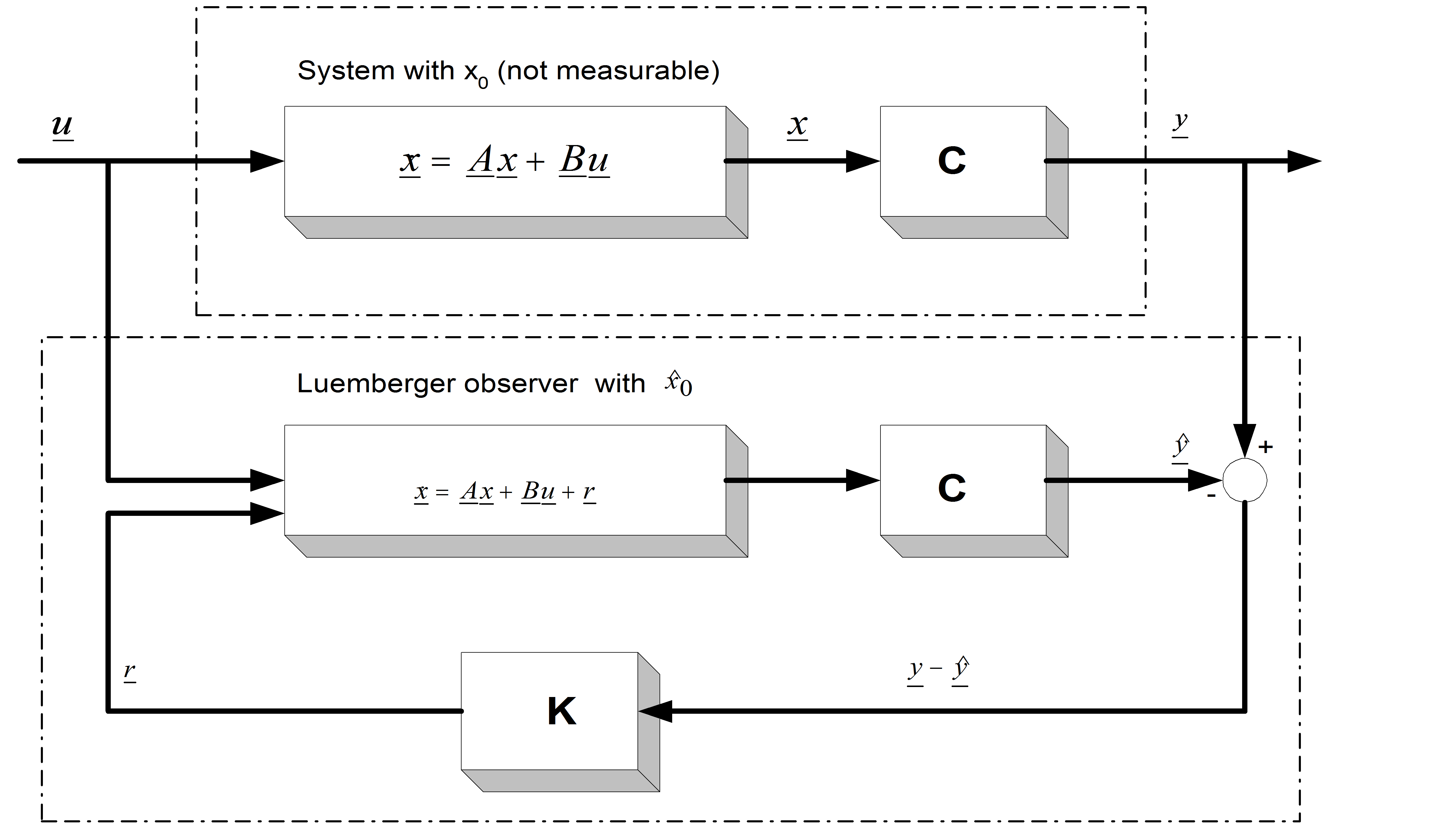
where u and y are the input and the output vectors and x is the state vector. A, B, and C are the system, input and output matrices. We measure the inputs and the outputs, but in most cases the states cannot be measured directly. If we need the value of a state variable (for example we want to control this state), we have to compute it from the measured quantities. In the case of asynchronous motors, we measure the currents and the voltages. We would like to control the speed of the rotor without any sensor (speed measurement means extra cost, may be technically impossible, etc.), that is, we would like to compute it from the measurements of the currents and of the voltages. It should be noted that the calculation of the states is not always possible (state observability), it depends on the system model [22]. An observer is used to determine the value of the states of a system. The general model of the state observer is shown in Figure 8.6 in the case of the LO, and Figure 8.5. in general case, for example, where  denotes the estimated state vector, L is the observer gain matrix, and a suitable way has to be chosen to make the output error r converge to zero. With a very simple approach we can realize a system that runs parallel to the real system, and calculates the state vector, as shown in Figure 85. This is based on the quite reasonable assumption that we know the input values of the system. This approach, however, does not take into account that the starting condition of the system is unknown, which is true in practically every case. This cause the state variable vector of the system model to be different from that of the real system. The problem can be overcome by using the principle that the estimated output vector is calculated based on the estimated state vector,
|
|
(,8.5) |

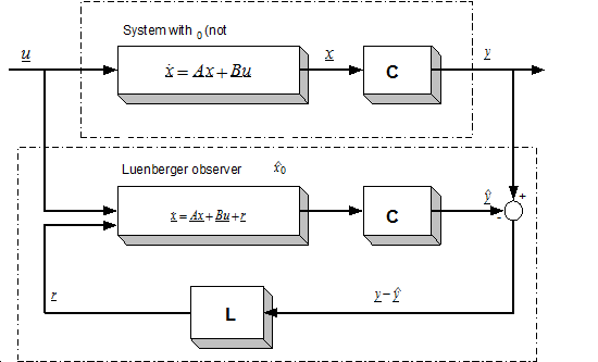
which may then be compared with the measured output vector. The difference will be used to correct the state vector of the system model. This is called the Luenberger Observer, and it can be seen in Figure 8.6. Now we can set up the state equation of the Luenberger Observer as follows:
|
|
(.8.6) |
Now we can ask how the matrix L must be set in order to make the error go to zero. Setting up a state equation for the error as follows does this:
|
|
(,8.7) |

where
|
|
(.8.8) |

If we now transpose the matrix of the error differential equation, we get a form which is very similar to a controller structure:
|
|
(.8.9) |
The effectiveness of such an observer greatly depends on the exact setting of the parameters, and on the exact measurement of the output vector. In the case of a real system, none of these criteria can be taken for granted. In the event of relatively great disturbances in the measurement, great parameter differences, or internal noises in the system, the Luenberger observer (as a deterministic case) cannot work anymore and we have to turn to the Kalman filter. Let us analyze the basics and the theory of the Kalman filter a little bit more because it is more important for our investigations, and its practical importance is much higher than that of a deterministic case.
8.3. The Kalman Filter Approach
The system we have considered up to now uses a sensor to measure the speed of the rotor. In many cases it is impossible to use sensors for speed measurement because it is either technically impossible or extremely expensive. As an example, we can mention the pumps used in oilrigs to pump out the oil. These have to work under the surface of the sea, sometimes at depths of 50 meters, and getting the speed measurement data up to the surface means extra cables, which is extremely expensive. It is clear that in such applications the most vulnerable part of the drives is the sensor. Cutting down the number of sensors and measurement cables provides a major cost reduction. Lately, there have been many proposals addressing this problem, and it has turned out that speed can be calculated from the measured current and voltage values of the AC motor. Some of these proposals are open loop solutions, which give some estimation of speed, but these solutions normally have a large error. For better results we need an observer or a filter, an estimator. The Kalman Filter has a good dynamic behavior, disturbance resistance, and it can work even in a standstill position. See [23] for a comparison of the performances of an observer, a Kalman Filter (KF) and an Extended Kalman Filter (EKF). Implementing a filter is a very complex problem, and it requires the model of the AC motor to be calculated in real time. Also, the Filter equations must be calculated, which normally means many matrix multiplication and one matrix inversion. Nevertheless, a processor with high calculation performance can fulfill these requirements. DSPs are especially well suited for this purpose, because of their good calculation-performance/price ratio. In low cost applications fixed point DSPs are desirable. The solution chosen by us is a Kalman filter, which is a statistically optimum observer (see exact details in [24]) if the statistical characteristics of the various noise elements are known. For the implementation of the Kalman Filter we need a much greater calculating capacity than that of the first generation C14 DSP, so at least a C50 DSP must be chosen to realize the field oriented control. This makes things more complicated of course, since the variables have to be scaled, which would be unnecessary with a floating-point processor. The Kalman filter is a special observer, which provides optimum filtering of the noises in measurement and inside the system if the covariance matrices of these noises are known. So let us first see what a stochastic estimator is.
8.4. Mathematical Background of Kalman Filters
When sampling the continuous-time and the discrete-time models of a system, it is very important to obtain the discrete time model of a plant or actuator, and, when needed, to apply an estimator or an observer to the system. A general state space model has the following equations in the continuous case:
|
|
(8.10) |
The calculation of the transfer function with Laplace transformation: Executing Laplace transformation of equations (8.10) we gain the following equations:
|
|
(.8.11) |
Rearranging equation (8.11) we get
|
|
(.8.12) |
Then the transfer function of the system is
|
|
(.8.13) |
Solving the state equation of the system by Laplace transformation:
For the inverse transformation we need the inverse of the term  . Let us first express this term in a geometrical series and we will see that in this case we can more easily effectuate the inverse transformation:
|
|
(.8.14) |
Applying the inverse Laplace transformation to the terms in the series we will get an infinite series, which is the Taylor series of  around 0:
|
|
(.8.15) |
The inverse Laplace transformation of equations (8.12) gives the solution for the state equations as follows:
|
|
(.8.16) |
8.4.1. Let us now descretize the continuous system:
We use the above treated continuous model for deducing the discrete model. The system is usually discretized by an A/D converter which can be considered as a zero order hold system. Using the notations t=tk+1, t0=tk , we get the following equation:
|
|
(,8.17) |
where  and T is the sampling period.
Let us introduce a new notation

,
and a new variable  , according to which
.
Introducing the above notations to (8.17) we get
|
|
(.8.18) |
The value of u is equal to the value of u(k) because of the ZOH. The value of  is constant, so both of them can be brought out from the integral:
|
|
(.8.19) |
After this the integral can be calculated or evaluated easily:
|
|
(.8.20) |
From (8.19) and (8.20) we get the state space equation of the discrete-time system:
|
|
(.8.21) |
The equation written in a matrix form is:
|
|
(,8.22) |
Where
|
|
(.8.23) |
From here on, we will work with discrete systems, so, for the sake of simplicity we will use the following notations for the state-space equation of the discrete-time system (it is very important that we do not mix the matrices A, B, C, D with those used in the case of the continuous system):
|
|
(,8.24) |
where
|
|
(.8.25) |
Let us now say a few words about the Gauss-Markov approximation, which is very important in defining the Kalman filter equations.
8.4.2. Gauss-Markov representation
The system without noises is described by equation (8.24), which can be given in a recursive form as
|
|
(,8.26) |
where  is the state transfer matrix.
In the time-variant case the  matrix is calculated as follows:

.
In the time-invariant case it will be
.
In the following we will try to deduce the equations in the time-invariant case, based on an iterative method. The time-variant case is similar, the only difference is in the  matrix:
|
|
(,8.27) |
Let us now give the time-variant equation charged by a Gauss distribution noise:
|
|
(,8.28) |
where  .
.
Equation (8.28) can be written in a recursive form just as before, in case of a noiseless system:
|
|
(.8.29) |
From the equations it can be seen that the values on the Markov representation depend only on the values of the precedent states. The values of the arbitrary x(k) will have a Gauss distribution because the next value is obtained with linear transformation of the previous values. Then the state space can be characterized by statistical measurement numbers like expected values and variance. Using the fact that the expected values of w and v vectors are zero, we will gain the following:
|
|
(,8.30) |
where  is expected value of the x vector, and
  is that of the y vector.
8.4.3. Auto-covariance of a stochastical system
Based on the definition of variance we get the following:
|
|
(,8.31) |
|
|
(,8.32) |

where  is the w noise variance. (in some literature noted by Q).
To simplify, let us introduce the following notation:
|
|
(.8.33) |
Evaluating the product of  we have
|
|
(.8.34) |
Because  and
and  are independent, their product will have an expected value around zero. Placing equation (8.34) back to the main equation we get
|
|
(.8.35) |

Similar steps for y lead to
|
|
(,8.36) |
|
|
(,8.37) |
where  is the v noise variance. (in some literature noted by R).
From the above equations it can be seen that the values of the x and y variables depend only on the previous states of the system. The above investigations are necessary for understanding the behavior and equations of the Kalman Filter, the operation of which is, in fact, a Gauss-Markov process.
8.4.4. Initial assumptions and the starting model
The model is the same as in the previous section. The only difference is that now we have a stochastic system, where w is the noise charging the state variable (system noise), and v is the noise charging the output variables (measurement noise). Both noises are Gauss white noises with zero expected values:
|
|
(,8.38) |
where:
as it was defined in (8.25).
Regarding the system noise w(k)
, (also Q in some literature)
and regarding the measurement noise v(k)
. (also R in some literature)
Because the two noises are independent,
.
The initial conditions of the linear stochastic difference equation (8.38) are

,
where R0, Rw, and Rv are positive semi-definite matrices.
8.5. The Equation of the Kalman Filter
8.5.1. The state estimator equations are
|
|
(.8.39) |

8.5.3. Determination of the error covariance matrix:
|
|
(8.42) |

From (8.41) we get the state variable covariance
|
|
(.8.43) |
From the initial condition it follows that the error covariance is 0, for any k. Therefore,
|
|
(.8.44) |
Using equation (8.44), we can simplify the function of P(k):
|
|
(.8.45) |
Minimalization of the covariance function using the K(k) matrix
The main task is to find the optimal K(k) matrix, which minimizes the  scalar, where
  is a vector, chosen arbitrarily.
Minimalization of the  scalar function
Where  is a symmetric positive semi-definit matrix and
  ,
,
|
|
(.8.46) |
Equation (8.46) can be minimized.
The function minimum is  ,
,
and this value is taken in the place of  .
.
Calculating the Kalman gain:
|
|
(.8.47) |
Equation (8.46) is the same as equation (8.47) if we introduce the following notations:
|
|
(.8.48) |

From the solution of equation (8.46) it follows that the value of Jk can be minimized and it can reach this value in the case of  .
.
Determination of the P(k+1) covariance matrix:
|
|
(.8.49) |

If we devise the calculation of the P matrix in two parts, then we get the prediction and correction phases, as will be presented as follow on.
8.5.4. Basic equations and the algorithms of the Kalman Filter
a.) Prediction phase:
|
|
(.8.50) |
b.) Calculation of the Kalman gain:
|
|
(.8.51) |
c.) Correction phase:
|
|
(.8.52) |
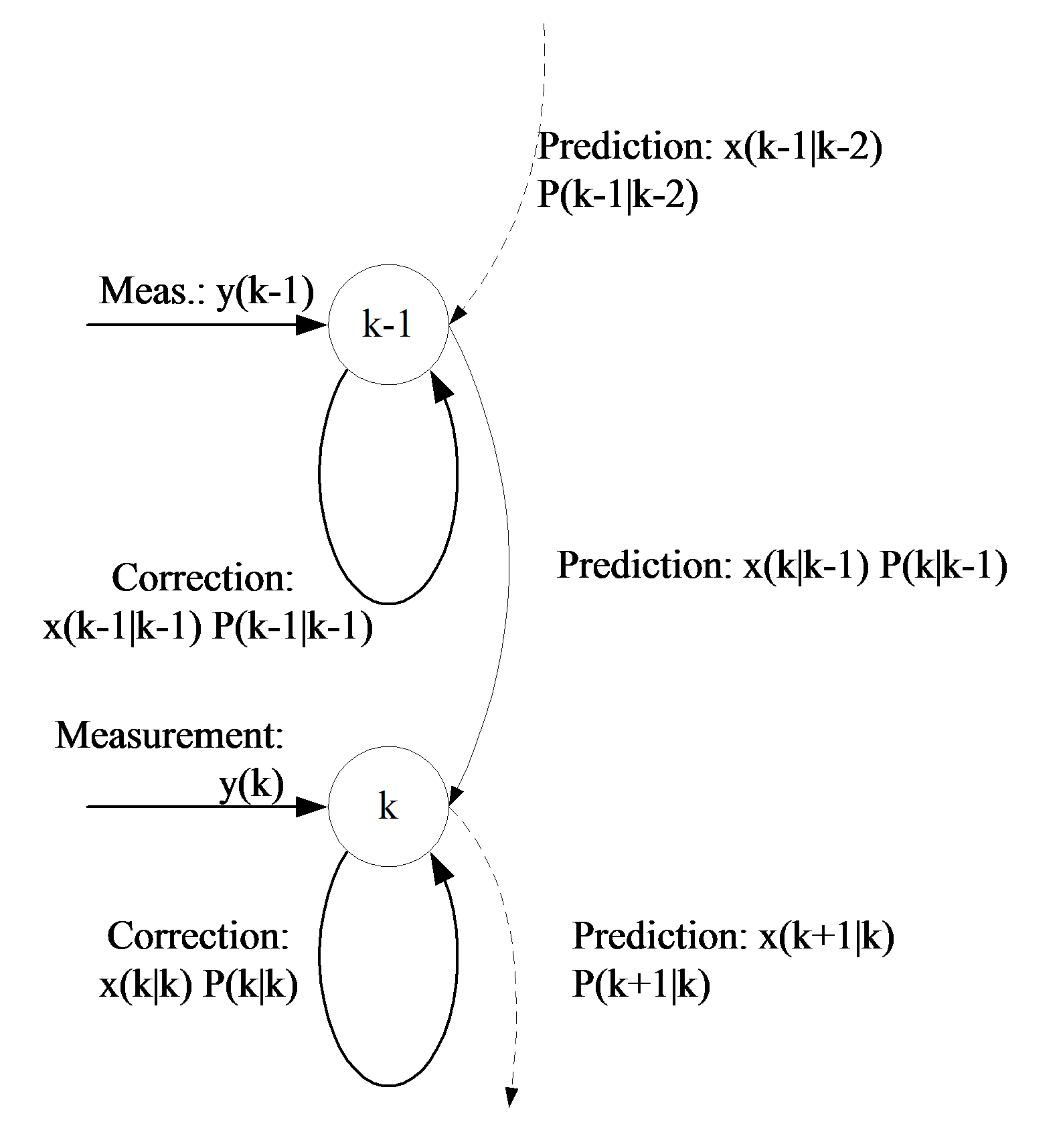
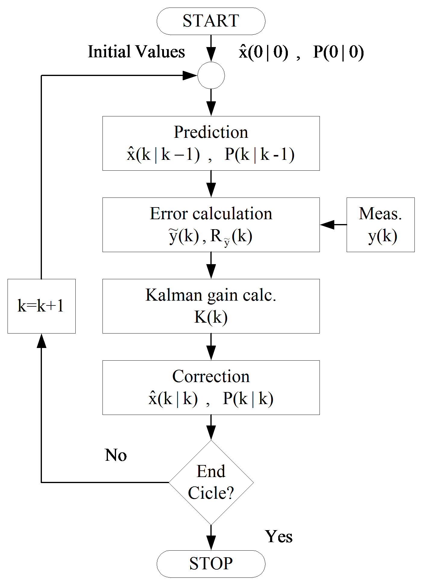
The functionality of these equations is shown in Figure 87. The Figure 88. shows the state flow of the Kalman Filter algorithm. As a first step, the state variable x must be chosen, and the initial value of the covariance matrix P must be given. After that the algorithm will estimate the value of the state variable in each sampling period, and determine the P matrix. Let us see step by step how it works properly.
Prediction phase: In this phase, according to equation (8.50), we calculate the value of the state variable vector and the intermediate values of the covariance matrix.
Calculation of error: From the calculated and measured values (y), we will determine the error of the estimation (8.51). This value is used afterwards to calculate the Kalman gain.
Correction phase: This is the last step of the algorithms. With the help of the Kalman gain (8.52) a more accurate x value will be determined and the final value of the covariance P matrix will be evaluated, too. These steps must be effectuated for every sampling period. A flow-chart of the algorithms’ functionality is presented in Figure 88.
8.5.5. Extended Kalman Filter
In case of the induction motor the state-space model is not linear because it contains the self-product of the state variables. So the KF treated above is not applicable, we have to turn to the extension of the KF which is also suitable for nonlinear systems. The essence of the method stems from linearization of the nonlinear model, which means that we use the first derivatives of the system and we will write the filter structure according to this. In the following, for the sake of simplicity, we will notate the vectors in the kth state with  ,
,  or
or  .
.  . The nonlinear system model in this case is
|
|
(,8.53) |
were  and
and  are nonlinear functions of
  . The
. The  and
and  functions will be approximated by Taylor series, and in this case we obtain a linear equation. The accuracy of the approximation depends on the grade of the Taylor series.
|
|
(,8.54) |
where the elements of matrices and
and  are the partial derivatives of
  and
and  according to
  :
:
|
|
(.8.55) |
We will use first order Taylor series, so we can neglect the higher order terms (HOTs), and, with the help of Taylor series, we can give the model in a linearized form:
|
|
(,8.56) |
where  .
.
Because the form of these equations is similar to that in the linear case, we can write the EKF equations according to equations (8.50), (8.51), and (8.52).
a.) Prediction phase:
|
|
(.8.57) |
b.) Kalman gain calculation:
|
|
(.8.58) |
c.) Correction phase:
|
|
(.8.59) |
Of course, in this case  and
and  are the covariances of the w and v noises. If we compare the equations, we can conclude that the only difference is in the A and C matrices.
8.6. Applicability of the Kalman Filter
The Kalman filter provides a solution that directly cares for the effects of the disturbance noises. The errors in the parameters will normally be handled as noise, too. Let us recall again the state-space model of the system with the following equations, and with practically accepted notations:
|
|
(,8.60) |
|
|
(,8.61) |
where r and are the system noise and the measurement noise. Now we assume that these noises are stationary, white, uncorrelated and Gauss noises, and their expected values are 0. Let us now define the covariance matrices of these noises:
|
|
(,8.62) |
|
|
(,8.63) |
where E{.} denotes the expected value. The overall structure of the Kalman filter is the same as that of the Luenberger observer in , the only difference being in the Kalman filter matrix K as it is shown in Figure 8-9. The system equations are also the same:
|
|
(.8.64) |
Let us introduce the reconstruction error  :
:
|
|
(.8.65) |
Following the substitutions as described earlier, we get:
|
|
(.8.66) |
Hence, if K is chosen so that the system in (8.66) is asymptotically stable, the reconstruction error will always converge to zero. If the model structure is given (e.g. a deterministic state space model described in previous chapter but the matrices A, B, and C depend on such parameters that can only be measured inaccurately or cannot be measured at all, these model parameters have to be estimated from the measurements of the input and the output values. A loss function is employed to measure the output error r shown in Figure 8-9. In the case of asynchronous motors, the state space model in fact is dependent e.g. on the rotor resistance Rr, which cannot be measured accurately and changes slowly as the temperature of the motor varies. The estimation of this parameter is very important because its accuracy greatly influences the performance of the control algorithm. We will follow the notations of [24], and denote the matrix of the Kalman filter by K. The only real difference between the Luenberger observer and the Kalman filter is in the setting of the K matrix. Doing this will be based on the covariance of the noises. We will first build the measure of the goodness of the observation, which is the following:
|
|
(.8.67) |

This depends on the choice of K. K has to be chosen to make J minimal. The solution of this is the following (see [23]):
|
|
(,8.68) |

where P can be calculated from the solution of the following equation (Ricatti):
|
|
(.8.69) |
Q and R have to be set up based on the stochastic properties of the corresponding noises. Since these are usually unknown, they are used as weight matrices in most cases. They are often set equal to the unit matrix, avoiding the need of deeper knowledge of the noises. In [24] a recursive algorithm is presented for the discrete time case to provide the solution for this equation. This algorithm is in fact the EKF (Extended Kalman Filter) algorithm, because the matrix of the Kalman filter, K, will be calculated on-line. The EKF is also capable of handling non-linear systems, such as the induction motor. In this case we do not have the optimum behaviour, which means the minimum variance, and it is also impossible to prove the convergence of the model. (See [25] and [23]). Let us now see the recursive form of the EKF as given in [19]. (This is basically the same as in , but with slightly different notations). All symbols in the following formulas denote matrices or vectors. They are not denoted with special notations because there is no possibility of mixing them up with scalars:
|
|
(,8.70) |

, (8.71)
|
|
(,8.72) |
|
|
(,8.73) |
|
|
(,8.74) |
where
|
|
(,8.75) |

|
|
(.8.76) |
These are the system vector and the output vector, respectively, and they can be explicitly calculated. The matrix K is the feedback matrix of the EKF. This matrix determines how the state vector of the EKF is modified after the output of the model is compared with the real output of the system. At this point it is important to mention that this system of equations contains many matrix operations, which can be difficult to implement in real-time. To implement this recursive algorithm, we will of course need the model of the motor, which means the matrices A, B, and C, from which we have to calculate the matrices and h. So, let us see again the motor model in this new context.
8.7. Motor model considerations
The most important thing in the following steps is the adaptation of the motor model to the Kalman Filter algorithms. This means that the motor equation must be included in the Kalman Filter model. The two main tasks are the following: first the estimation of the rotor speed, then the estimation of rotor resistance. For estimating the speed, two different co-ordinate systems will be used:
Stationary two-phase co-ordinate system, fixed to the stator;
Rotating co-ordinate system, fixed to the rotor flux.
8.7.1. Estimating the rotor speed
For parameter estimation the equations of the motor model must be given in discrete form. Looking at previous chapter it can be realized that the motor model was deduced in the continuous case, so it is now necessary to give the model in the discrete case. During discretization the higher order terms are neglected because the square of the sampling time or its values at a higher power are approximately zero. So the discrete model state matrix (“A” matrix) corresponds to the sum of the continuous model A matrix multiplied by the sampling time (T) added to the unity matrix. The discrete time “B” matrix is nothing else but the continuous time „B” matrix multiplied by the sampling time (T). In the equation  is the discrete time state matrix and
  is the discrete time „B” matrix. The model of the AC motor, as it was analyzed before is based mostly on [19], [26], and [25].
|
|
(8.77) |

In the following the „A” and „B” matrices symbolize the discrete ones, and, according to these, the motor model will have the form as follows:
|
|
(.8.78) |
8.7.2. Estimation of speed on the stationary reference frame
Equation (8.78) is the starting or reference equation, which was used during the estimation and has been adapted to the Kalman Filter (KF). The KF is applicable to predict or estimate only the state variables of the model, so the speed of the rotor  must be included in the set of state variables. We do not give a formula for calculating the speed
  , we only use the assumption that
  , which is a good approximation during one sampling period. Therefore, in the prediction phase, the speed values are identical with the values in the previous state. In the correction phase, the rotor speed will be modified according to the measured
  values (see equation (8.53) ). Further, because
  is included in the state variable matrix, the model is not linear anymore, so we have to turn to the extended Kalman Filter. In this case, the general equation of the model has been changed slightly because of the nonlinearities:
|
|
(.8.79) |
In the case of the motor model, there is a linear relationship between the output ( ) and the input (
 ), and this is why the C matrix is used instead of the “g” function (8.53). The state model in the nonlinear case is the following:
|
|
(.8.80) |
Let us analyze the nonlinear „f” function:
|
|
(8.81) |
We do not need to give the “g” function in the model because the C matrix is linear. To effectuate the estimation, we further need the partial derivatives of the function “f”. This matrix is sometimes denoted by „A”, and in this case the equations are very similar to the equations in the case of a linear filter.
|
|
(8.82) |
In the calculation of the y we use linear equations:
|
|
(8.83) |
These equations will go into the equations of the Kalman Filter.
8.7.3. Estimation of speed in a rotating reference frame
In this section we will estimate the rotor speed in a d-q reference frame fixed to the rotor flux. The equations are borrowed from the FOC control of induction motors, and are extended with the motion/kinetic equation of the motor. The advantage of this method is that the speed is approximated according to the motion equation, which is done in the prediction phase, and then followed by a correction, which is done with the help of the measured data. In the previous case of the α- stationary co-ordinate system we did not use the motion equation, so in the present case the filter structure is more complex than it was in the previous case. Let us see the new state variables and the model itself. The magnetizing current, which was dealt with in previous chapter in the case of FOC , has appeared as a state variable In this case the estimation is based on the following equations. The first three are the stator current equations in a d-q co-ordinate system and the fourth one is the kinetic equation:
|
|
(,8.84) |

|
|
(,8.85) |
|
|
(,8.86) |
|
|
(,8.87) |
It can be observed that the last equation contains the product of the q component of the stator current and the magnetizing current. Let us now identify again the state variables, the inputs and the outputs. The state variable is a 4th order vector, containing the stator current components, the magnetizing current, and the speed of the rotor. The output (y) of the filter is the α- stationary components of the stator current vector. The stator voltage is the input of the model.
|
|
(8.88) |
Equation (8.87) has been deduced from the equation borrowed from the modelling of asynchronous motor, which is the basic kinetic equation of the motor. It can easily be observed that the speed of the motor depends intensively on the electromagnetic torque and the load torque. The load torque is one input of the model and can be considered as a disturbance: The electromagnetic torque expression has been presented also in previous chapter and these equations will be repeated here for convenience:
![]() is the rotor flux speed in the stationary reference frame. For the calculation of the speed we can proceed in two ways:
is the rotor flux speed in the stationary reference frame. For the calculation of the speed we can proceed in two ways:
a) ![]() ,as a constant:
,as a constant:
The essence of this method relies on the equation below, where we consider the rotor flux speed as a constant value and we calculate the slip and the rotor speed outside the KF. This approach considerably simplifies the system model:  .
.
Let us see what it looks like:
|
|
(.8.89) |
The partial derivative matrix of „f” is the following:
|
|
(8.90) |

b) ![]() inserted into the filter model:
inserted into the filter model:
In this case we use (8.91) equation for calculating ![]() :
:
|
|
(,8.91) |
The equation has three state variables: the magnetizing current, the “q” component of the stator current, and the speed of the rotor. These state variables will complicate the model and the partial derivatives matrix of “f”. Another draw-back of this method is that if the magnetizing current is zero, the value of ![]() cannot be determined. This means that we have to check the value of the magnetizing current in each sampling period. Let us see now the form of the „f” function and its partial derivatives in these circumstances:
cannot be determined. This means that we have to check the value of the magnetizing current in each sampling period. Let us see now the form of the „f” function and its partial derivatives in these circumstances:
|
|
(8.92) |
|
|
(8.93) |
The input of the model in both cases is the stator voltage, in a stationary reference frame.
8.7.4. Estimating the rotor resistance
Until now the value of the rotor resistance has been considered as a constant, and the model of the motor has been deduced according to this assumption. It is well known that during motor operation this value can change considerably, and this depends to a great extent on the internal temperature of the motor. To give an analytical equation to these considerations is very difficult, so we will consider these factors as noise in the system. Mostly in the range of low speed operation (where the temperature of the motor increases), the value of the rotor resistance does not absolutely match with its constant value. In this case we use a KF filter to approximate the value of the rotor resistance and to increase the accuracy of the model. Let us see now how this is implemented. The rotor flux speed is not introduced in the filter model. The estimation of Rr can be effectuated also for the second case b) above, the steps are the same. Now we have to include Rr in the state variable matrix as shown below:
|
|
(.8.94) |
The output and the input of the system are kept as before. The rotor time constant has been extracted from the formula of the function “f” because this term depends on the rotor resistance:
|
|
(.8.95) |

Inserting the „f” function into equation (8.92) we will have the following formula:
|
|
(.8.96) |
As it can be seen, we do not give any formulae for calculating Rr, which, from the point of view of the filter, means that we do not have a prediction phase. Therefore, the value of Rr is identical with its previous value in the prediction phase (8.57). The approximation of Rr is made by the KF in the correction phase. The matrix of partial derivatives of the function „f” will be
|
|
(.8.97) |
These formulae will be inserted into the model of the filter. This will be the last step to enable both real-time implementation and simulation. Let me now summarize the main design steps for a speed-sensorless induction motor drive implementation using the discretized EKF algorithm.
The steps which sould be made are as follows:
-
Selection of the time-domain induction machine model;
-
Discretization of the induction machine model;
-
Determination of the noise and state covariance matrices , R, P;
-
Implementation of the discretized EKF algorithm; tuning.
The above design steps will be shortly discussed:
1. For the purpose of using an EKF for the estimation of the rotor speed of an induction machine, it is possible to use various machine models. For example, it is possible to use the equations express in the rotor-flux-oriented reference frame, or in the stator-flux-oriented reference frame. When the model expressed in the rotor-flux-oriented reference frame is used, the stator current components in the rotor-flux-oriented reference frame are also state variables and the input and output matrices contain the sine and cosine the angle of the rotor flux-linkage space vector. These transformations introduce extra non-linearities, but these transformations are not present in the model established in the stationary reference frame. The main advantages of using the model in the stationary reference frame are:
-
Reduced computation time (e.g. due to reduced non-linearities);
-
Smaller sampling times;
-
Higher accuracy;
-
More stable behavior.
2. The discretization of the model has been treated extensively previously so in this place we omit the treatment again.
3. The goal of the Kalman filter is to obtain unmeasurable states (rotor speed) by using measured states, and also statistics of the noise and measurements (covariance matrices Q,R,P of the system noise vector, measurement noise vector, and system state vector respectively). In general, by means of the noise inputs, it is possible to take account of computational inaccuracies, modelling errors, and errors in the measurements. The filter estimation is obtained from the predicted values of the states and this is corrected recursively by using a correction term, which is the product of the Kalman gain and the deviation of the estimated measurement output vector and the actual output vector.The Kalman gain is chosen to result in the best possible estimated states. Thus the filter algorithm contains basically two main stages, a prediction stage and a filtering stage. During the prediction stage, the next predicted values of the states are obtained by using a mathematical model (state-variable equations) and also the previous values of the estimated states. Furthermore, the predicted state covariance matrix (P) is also obtained before the new measurements are made, and for this purpose the mathematical model and also the covariance matrix of the system (Q) are used. In the second stage, which is the filtering stage, the next estimated states, are obtained from the predicted estimates by adding a correction term  to the predicted value. This correction term is a weighted difference between the actual output vector and the predicted output vector where K is the Kalman gain.
Thus the predicted state estimate (and also its covariance matrix) is corrected through a feedback correction scheme that makes use of the actual measured quantities. The Kalman gain is chosen to minimize the estimation-error variances of the states to be estimated. The computations are realized by using recursive relations. The algorithm is computationally intensive, and the accuracy also depends on the model parameters used. A critical part of the design is to use correct initial values for the various covariance matrixes.
These can be obtained by considering the stochastic properties of the corresponding noises. Since these are usually not known, in most cases they are used as weight matrices, but it should be noted that sometimes simple qualitative rules can be set up for obtaining the covariances in the noise vectors. The system noise matrix Q depending on the model is a five-by-five matrix, the measurement noise matrix R is a two-by-two matrix, so in general this would require the knowledge of 29 elements. However, by assuming that the noise signals are not correlated, both Q and R are diagonal, and only 5 elements must be known in Q and 2 elements in R. However, the perameters in the direct and quadrature axes are the same, which means the two first elements in the diagonal of Q (q11=q22) are equal, the third and fourth elements in the diagonal of Q (q33=q44) are equal so Q=diag(q11,q11,q33,q33,q55) contains only 3 elements which have to be known. Similarly, the two diagonal elements in R (r11=r22) are equal, thus R=diag(r11,r11). It follows that in total only 4 noise covariance elements must be known.
As discussed above, the EKF is an optimal, recursive state estimator, and the EKF algorithm contains basically two main stages, a prediction stage and a filtering stage. The EKF equation is:
|
|
(8.98) |
The structure of the EKF is shown in Figure 8-10.
The starting-state covariance matrix can be considered as a diagonal matrix, where all the elements are equal. The initial values of the covariance matrices reflect on the degree of knowledge of the initial state: the higher their values, the less accurate is any available information and the convergence speed of the estimation process will increase. However, divergence problems, or large oscillation of state estimates around a true value may occur when too high initial covariance values are chosen. A suitable selection allows us to be obtain satisfactory speed convergence, and avoids divergence problems or unwanted large oscillations.
The accuracy of the state estimation is affected by the ammont of information that the stochastic filter can extract from its mathematical model and the measurement data processing. Some of the estimated variables, especially unmeasured ones, may indirectly and weakly be linked to the measurement data, so only poor information is available to the EKF. Finally it should be noted that another important factor which influences the estimation accuracy is due to the different size of the state variables, since the minimization of the errors for the variables with small size. This problem can be overcome by choosing normalized state-variables. For the realization of the EKF algorithm it is very convenient to use a signal processor (e.g. Texas Instruments TMS320C30, TmS320C40, TMS320C50, etc.), due to the large number of multiplications required and also due to fact that all of the computations have to be performed fast: within one sampling interval. The calculation time of the EKF is 130  s on the TMS320C40. However, the calculation times can be reduced by using optimized machine models.
The EKF described above can be used under both steady-state and transient conditions of the induction machine for the estimation of the rotor speed. By using the EKF in the drive system, it is possible to implement a PWM inverter-fed induction motor drive without the need of an extra speed sensor. It should be noted that accurate speed sensing is obtained in a very wide speed-range, down to very low values of speed (but not zero speed). However, care must be taken in the selection of the machine parameters and covariance values used. The speed estimation scheme requires the monitored stator voltages and stator currents. Instead of using the monitored stator line voltages, the stator voltages can also be reconstructed by using the d.c. link voltage and inverter switching states, but especially at low speeds it is necessary to have an appropriate dead-time compensation, and also the voltage drops across the inverter Switches (e.g. MOSFETs, IGBTs) must be considered. Furthermore in a VSI inverter-fed vector-controlled induction motor drive, where a space-vector modulator is used, it is also possible to use the reference voltages (which are the inputs to the modulator) instead of the actual voltages, but this requires appropriate error compensation.
The tuning of the EKF involves an iterative modification of the machine parameters and covariance in order to yield the best estimates of the states. Changing the covariance matrices Q and R affects both the transient duration and steady-state operation of the filter. Increasing Q corresponds to stronger system noises, or larger uncertainty in the machine model used. The filter gain matrix elements will also increase and thus the measurements will be more heavily weighted and the filter transient performance will be faster. If the covariance R is increased, this corresponds to the fact that the measurements of the currents are subjected to a stronger noise, and should be weight less by the filter. Thus the filter gain matrix elements will decrease and this results in slower transient performance. Finally it should be noted that in general, the following qualitative tuning rules can be obtained: Rule 1: If R is large then K is small (and the transient performance is faster). Rule 2: If Q is large then K is large (and the transient performance is slower). However, if Q is too large or if R is too small, instability can arise. In summary it can be stated that the EKF algorithm is computationally very intensive, but it can also be used for joint state and parameter estimation. It should be noted that to reduce the computational effort and any steady state error, it is possible to use various EKFs, which utilize reduced-order machine models and different reference frames (e. g. a reference frame fixed to the stator current vector).
8.8. Realization of the Kalman Filter
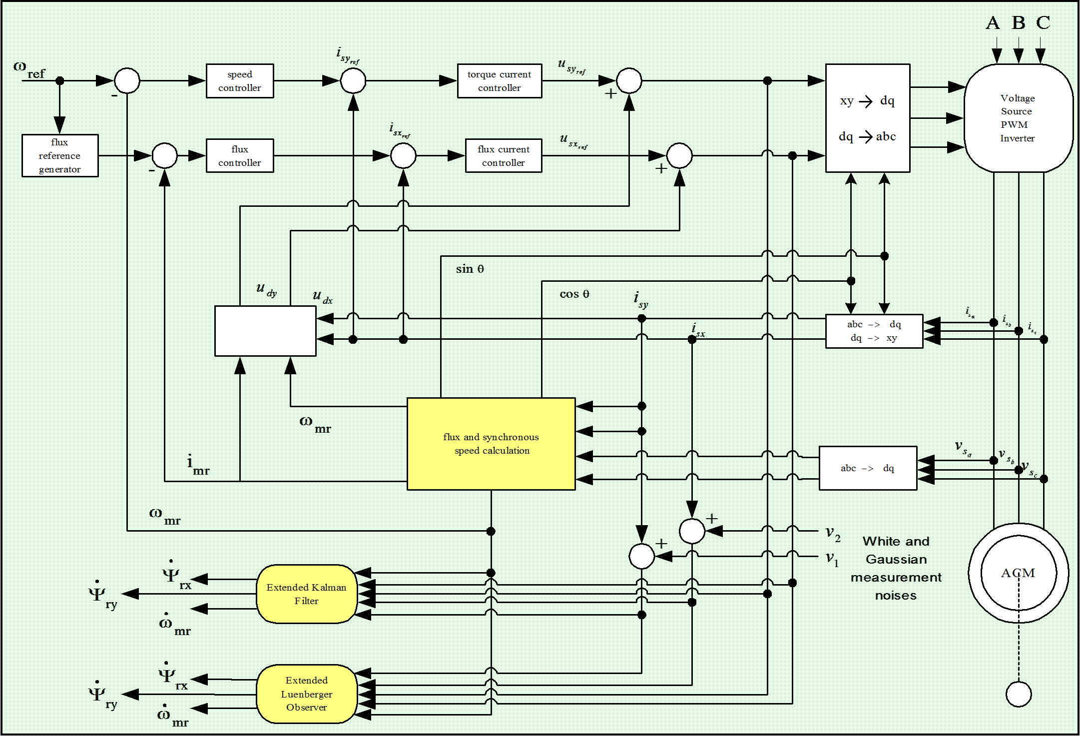
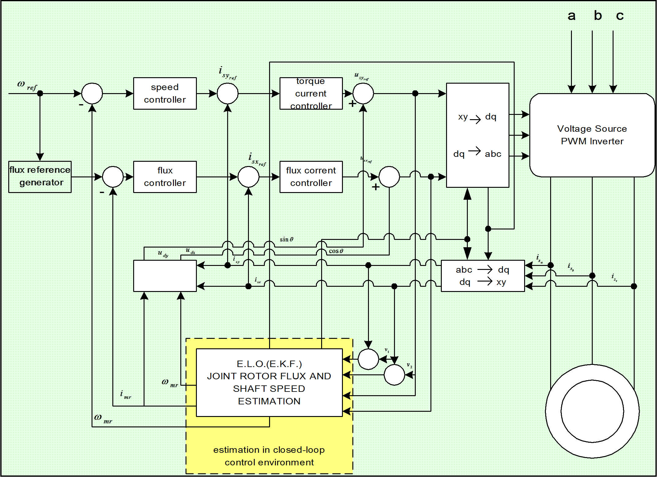
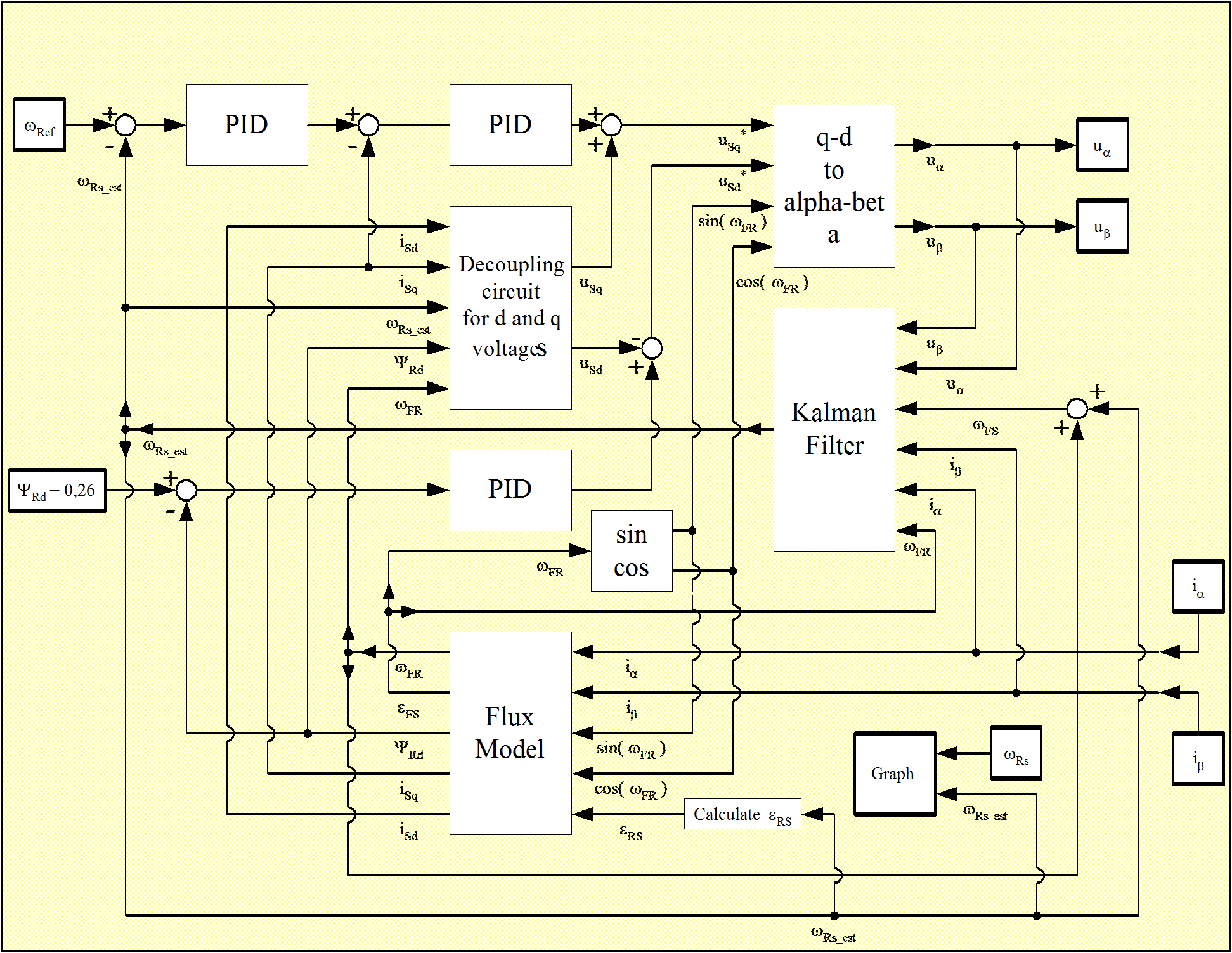
Reaching this point, the realization of the model in Matlab/Simulink can begin. The strategy for implementing the Kalman Filter based method was the following: before introducing the filter on the feed-back line, first we used off-line identification methods as shown in Figure 8-11. [25]. As it can be seen on the figure, a traditional FOC method was used for testing the performance of the estimation. When the estimated values match the values of the system, the observers can be inserted in the feedback loop for achieving the on-line identification of the desired parameters. In the closed loop environment both the rotor flux and the rotor’s angular speed are also estimated, so we do not need any flux model or flux calculation procedure. The realized model structure can be seen in Figure 8-12. Realizing the complete Kalman filter as a Simulink model would have resulted in a very complicated model, and it seemed easier to implement it simply as a Matlab language file. Another advantage of this is that the Matlab language file can more easily be converted into an assembly program. A subsystem was inserted into the system that contains the Kalman filter, which is then built into the model as an S-function. The overall structure of the controller has not been changed very much. The filter is in the subsystem called KF. Its output depends on which model we use. The Figure 8-13. shows the case of the EKF with the second motor model from [19]. In this case, the outputs of the system are all state variables: the rotor fluxes, the stator currents, and the rotor speed. The inputs are measured rotor currents and rotor voltages. In the other case, the output would be only the rotor speed, but the estimated rotor speed would be needed as well, which sould be calculated by a flux model.
These tests reveal that the model of Vas presented in [26] has a much more stable behavior. After achieving the required simulation results, real-time implementation could begin, based again on the second model.