Chapter 7. Modelling Induction Motors
Prev		Next

Chapter 7. Modelling Induction Motors

Table of Contents

7.1. The AC Induction Motor

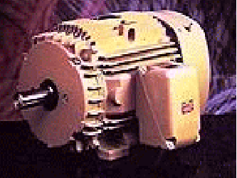
Asynchronous motors are based on induction. The least expensive and most widely spread induction motor is the so-called ‘squirrel cage’ motor. A typical asynchronous motor is shown in Figure 7-1. A metal ring at the ends resulting in a short circuit connects the wires along the rotor axis. There is no current supply needed from outside the rotor to create a magnetic field in the rotor. This is the reason why this motor is so robust and inexpensive. The stator phases create a magnetic field in the air gap rotating at the speed of the stator frequency (1).

Figure 7.1. An asynchronous motor

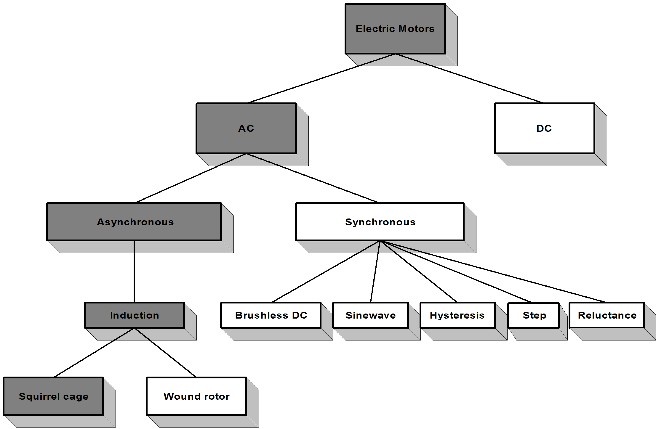
The changing field induces a current in the cage wires, which then results in the formation of a second magnetic field around the rotor wires. As a consequence of the forces created by these two fields, the rotor starts rotating in the direction of the stator field but at a slower speed (). If the rotor revolved at the same frequency as the stator, then the rotor field would be in phase with the stator field and no induction would be possible. The difference between the stator and the rotor frequency is called slip frequency (slip= 1-). There are several ways to control an induction motor in torque, speed or position, which can be categorized into two groups: there are scalar and vector control methods. Because of its outstanding robustness among all AC Motors, as can be seen in the Figure 7-2., the asynchronous ‘squirrel cage’ induction motor was chosen for detailed analysis and for control purposes. Further, the experimental application of this motor type has growing significance.

Figure 7.2. Classification of electric motors

The following section will briefly describe this motor with the purpose of a deeper insight into its behavior later on.

7.2. General equations of AC Motors

The asynchronous or AC induction motor is represented by a stator and a concentric rotor with three-phase windings and a narrow airgap between the smooth surfaces of the rotor and the stator. Only the stator windings are fed by a voltage or current source inverter. The connection between the stator and the rotor is made by the flux, which means there is no mechanical connection between them apart from the bearings. For deducing the general equations of the AC induction motor (with “squirrel cage” rotor), let as make the following assumptions:

Figure 7.3. Sinusoidal Current density distribution

Presume a symmetrical three-phase windings system in the machine.

neglect the cooper losses and the slots in the machine;

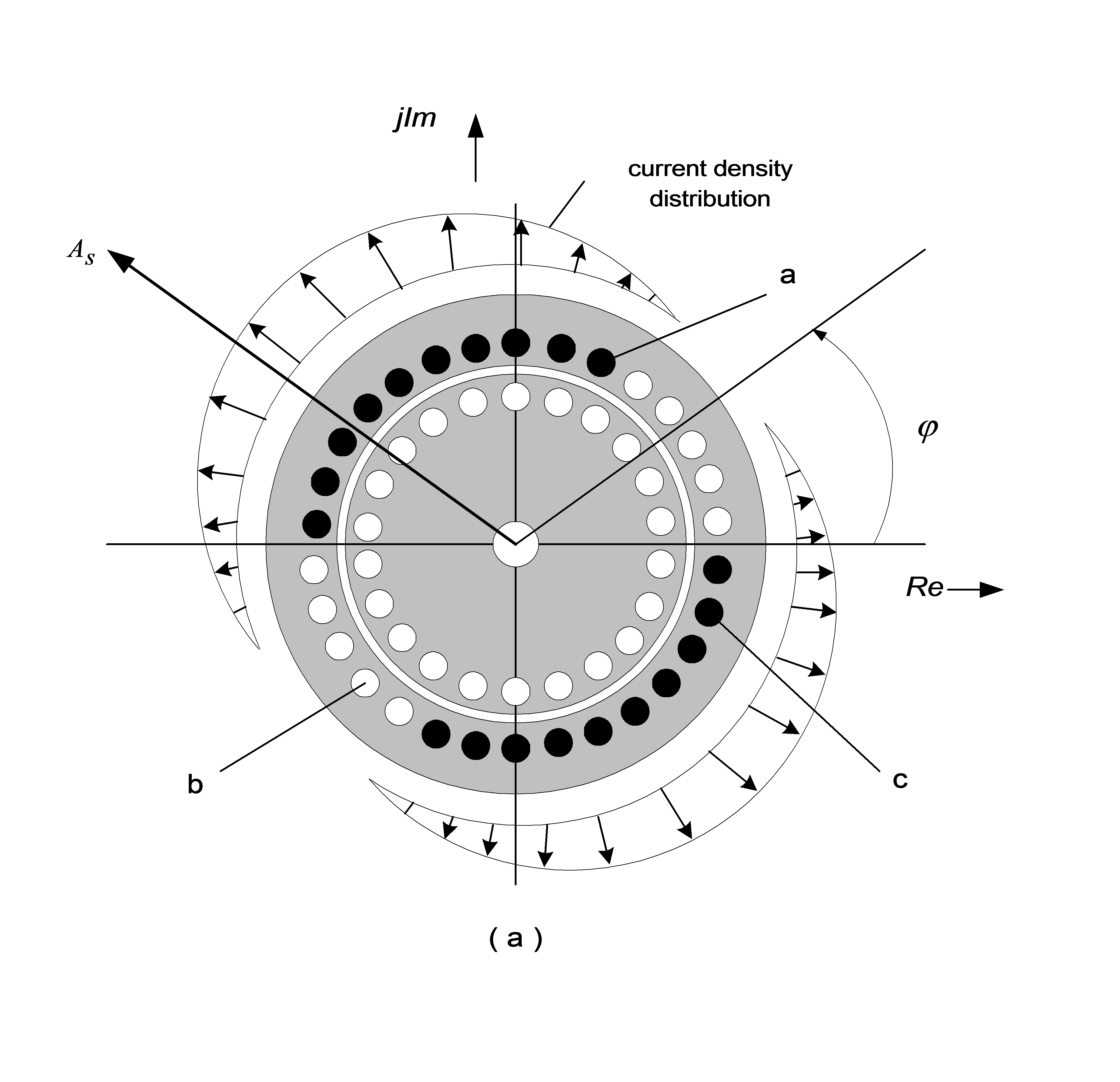
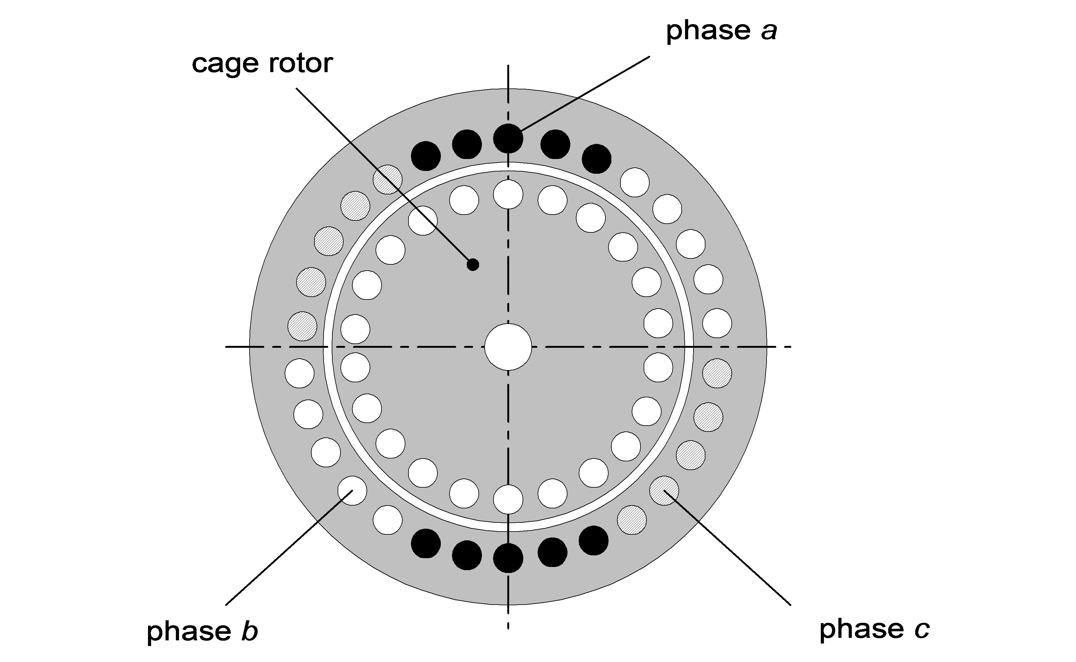
spatial distribution of fluxes and amperturns wave are considered sinusoidal, as can be seen in Figure 7-3, the cross section of an Induction motor is shown in Figure 7-4.;
all the calculations based on the three-phased vector theory;
all the losses due to wiring, saturation, and slot effects can be neglected;
stator and rotor permeability are assumed to be infinite.

Figure 7.4. Cross section of an Induction Motor

7.2.1. Machine equations in a natural co-ordinate system

The voltage equations of the stator are the following:

$U_{s a} = i_{s a} \cdot R_{s a} + \frac{d Ψ_{s a}}{d t}$

(7.1)

$U_{s b} = i_{s b} \cdot R_{s b} + \frac{d Ψ_{s b}}{d t}$

(7.2)

$U_{s c} = i_{s c} \cdot R_{s c} + \frac{d Ψ_{s c}}{d t}$

(7.3)

where $Ψ_{a}, Ψ_{b}, Ψ_{c}$ are the total fluxes of each phase including the main field of the windings and the leakage flux connection with the other windings, and $R_{a} = R_{b} = R_{c} = R_{s}$ is the one phase winding resistance. If we describe the above equations (7.1)(7.2)(7.3) according to the vector theory, the stator vectorial voltage equation will be the following:

${\bar{U}}_{s} = {\bar{i}}_{s} \cdot R_{s} + \frac{d {\bar{Ψ}}_{s}}{dt}$

(7.4)

$U_{s}_{0} = i_{0} \cdot R_{s} + \frac{{dΨ}_{s}_{0}}{dt}$

(7.5)

where the latter equation is the zero sequence component.

Figure 7.5. Three-phase stator and rotor windings of an asynchronous motor in the natural coordinate system

In practice, the zero sequence component can be neglected, so the equation (7.5) can be ignored and only one vectorial equation will describe the motor behavior instead of three phase equations. Writing the equation for rotor windings and proceeding like before we can easily obtain the vectorial voltage equation of the rotor:

${\bar{U}}_{r} = {\bar{i}}_{r} \cdot R_{r} + \frac{d {\bar{Ψ}}_{r}}{d t}$

(7.6)

$U_{r 0} = i_{r 0} \cdot R_{r} + \frac{d Ψ_{r 0}}{d t}$

(7.7)

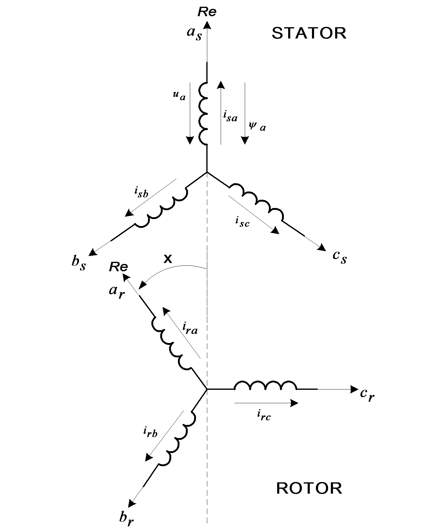
where, for the same reason as before, the equation (7.7) can be ignored. The currents circulating in the three stator and three rotor windings generate the fluxes in the motor. We suppose that the air-gap is constant and the spatial distribution of the main magnetic field is sinusoidal, so the mutual inductance is proportional with the cosine value of the angle between two windings. Let us choose the real axes of the complex plane to match with the “a” phase axes. In the following discussion, we will call Natural Co-ordinate System the complex co-ordinate system fixed in this way to the “abc” axes of the motor. According to this agreement, the flux of phase “a” of the stator flux vector will be given by the equation (7.8), (7.9):

${\bar{Ψ}}_{s} = {\bar{i}}_{s} \cdot L_{s} + {\bar{i}}_{r} \cdot e^{^{j x}} \cdot L_{m}$

(7.8)

${\bar{Ψ}}_{r} = {\bar{i}}_{s} \cdot e^{- j x} \cdot L_{m} + {\bar{i}}_{r} \cdot L_{r}$

(7.9)

The motor’s general equations are defined by (7.4), (7.6), (7.8), (7.9). If $u_{s}, u_{r}$ are given and the time function $x (t)$ is also given, then the above equations unambiguously define the motor currents. They form a linear differential equation system with time dependent coefficients. If $x (t)$ is not known or not given and must be calculated from the torque or motion equation, then the above equation system becomes nonlinear. The $e^{j x}$ factor from the flux equations should be eliminated if the stator and rotor quantities are evaluated in the same co-ordinate system.

7.2.2. Machine Equations in a common co-ordinate system

In the previous section the stator quantities were given in their own complex co-ordinate system with the real axes fixed to the “a” phase axes of the stator windings. Let the $x_{k} (t)$ function describe the angular position of the new common co-ordinate system, referring to the fixed “a” phase axes. In this new common co-ordinate system the ${\bar{i}}_{s}$ stator current vector angle, written as a complex number, became $α^{*}$ instead of the former $α$ . So this angle can be expressed as * = - xk.

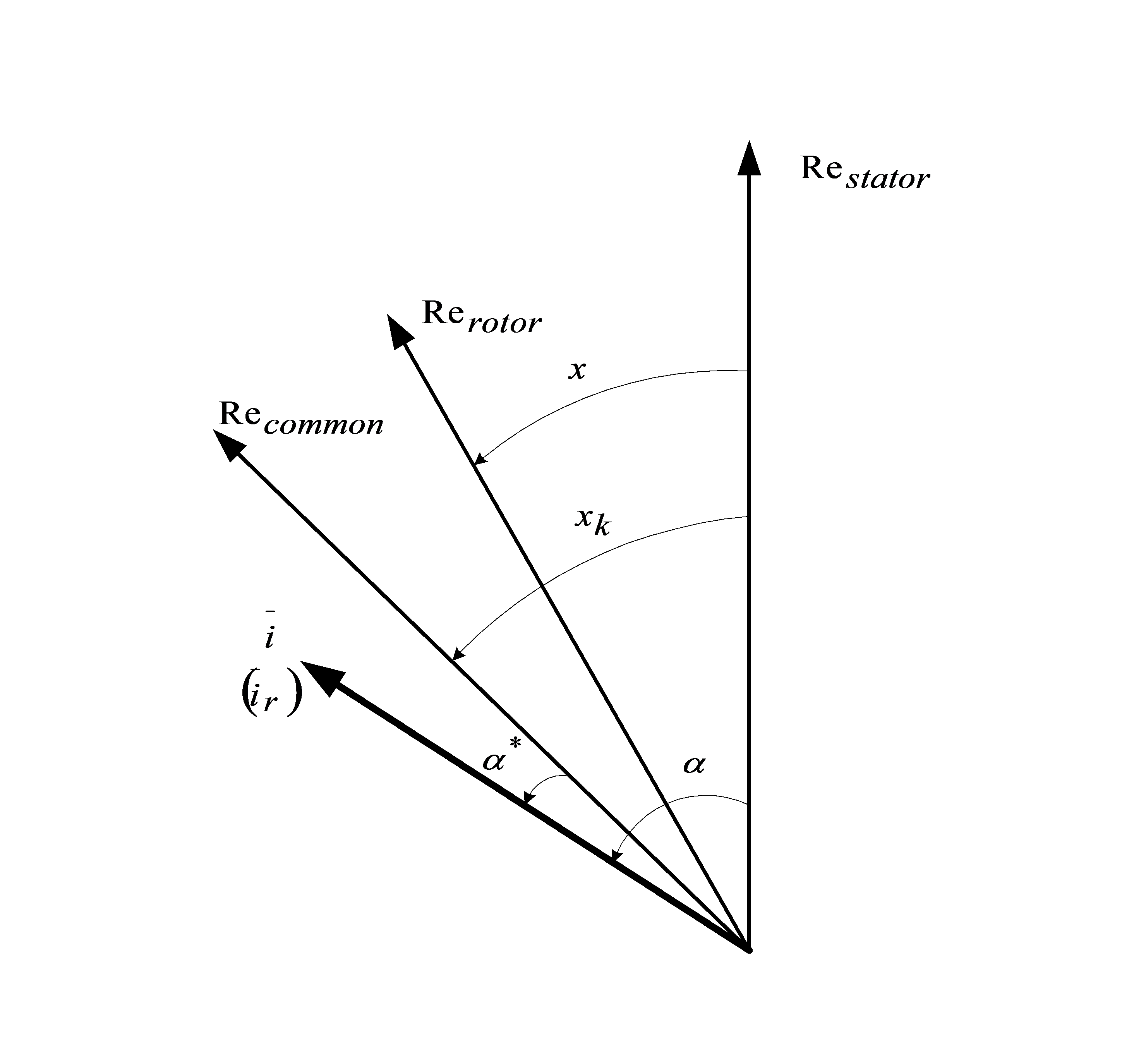
Figure 7.6. The coordinate systems for machine equation transformation

Now if we denote the current vector with ${\bar{i}}_{s}^{*}$ in the new reference frame, then the stator quantities can be expressed as

${\bar{i}}_{s}^{*} = {\bar{i}}_{s} \cdot e^{- j x_{k}}$

(7.10)

${\bar{i}}_{s} = {\bar{i}}_{s}^{*} \cdot e^{j x_{k}}$

(7.11)

The angle between the two (fixed to the stator, common) co-ordinate systems is xk-x, so the rotor quantities can be expressed as

${\bar{i}}_{r}^{*} = \bar{i_{r}} \cdot e^{- j (x_{k} - x)}$

(7.12)

${\bar{i}}_{r} = {\bar{i}}_{r}^{*} \cdot e^{j (x_{k} - x)}$

(7.13)

Having expressed the old quantities of the flux equation, in the new co-ordinate system, after a few simplifications, we obtain the following flux equations in the new common co-ordinate system:

${\bar{Ψ}}_{s}^{*} = {\bar{i}}_{s}^{*} \cdot L_{s} + {\bar{i}}_{r}^{*} \cdot L_{m}$

(7.14)

${\bar{Ψ}}_{r}^{*} = {\bar{i}}_{s}^{*} \cdot L_{m} + {\bar{i}}_{r}^{*} \cdot L_{r}^{}$

(7.15)

If we look carefully at these equations, we can observe that the time dependent coefficients are not present in the equations anymore. So the flux equations of the asynchronous motor became as simple as in the case of a transformer. Let us have a look at the voltage equations, because they have become slightly complicated:

$\frac{d {\bar{Ψ}}_{s}}{d t} = \frac{d ({\bar{Ψ}}_{s}^{*} \cdot e^{j x_{k}})}{d t} = \frac{d {\bar{Ψ}}_{s}^{*}}{d t} \cdot e^{j x_{k}} + j \frac{d x_{k}}{d t} \cdot {\bar{Ψ}}_{s}^{*} \cdot e^{j x_{k}}$

(7.16)

$\frac{d {\bar{Ψ}}_{r}}{d t} = \frac{d ({\bar{Ψ}}_{r}^{*} \cdot e^{j (x_{k} - x)})}{d t} = \frac{d {\bar{Ψ}}_{r}^{*}}{d t} \cdot e^{j (x_{k} - x)} + j (\frac{d x_{k}}{d t} - \frac{d x}{d t}) \cdot {\bar{Ψ}}_{r}^{*} \cdot e^{j (x_{k} - x)}$

(7.17)

where dx/dt = is the rotor speed or angular velocity, and dxk/dt=k is the speed or angular velocity of the co-ordinate system. Both of these should be time dependent variables.

${\bar{u}}_{s}^{*} = {\bar{u}}_{s} \cdot e^{- j x_{k}} = {\bar{i}}_{s} \cdot e^{- j x_{k}} \cdot R_{s} + \frac{d {\bar{Ψ}}_{s}}{d t} \cdot e^{- j x_{k}} = {\bar{i}}_{s}^{*} \cdot R_{s} + \frac{d {\bar{Ψ}}_{s}^{*}}{d t} + j ω_{k} \cdot {\bar{Ψ}}_{s}^{*}$

(7.18)

$\bar{u_{r}^{*}} = \bar{i_{r}} \cdot e^{- j (x_{k} - x)} \cdot R_{r} + \frac{d \bar{Ψ_{r}}}{d t} \cdot e^{- j (x_{k} - x)} = \bar{i_{r}^{*}} \cdot R_{r} + \frac{d \bar{Ψ_{r}^{*}}}{d t} + j (ω_{k} - ω) \cdot \bar{Ψ_{r}^{*}}$

(7.19)

Looking at these equations we can see that the time dependent coefficients are present in the voltage equations, due to $ω_{k}, (ω_{k} - ω)$ . Supposing that the speed of the rotor in most cases is constant or cannot change dramatically, and choosing a co-ordinate system with a constant speed we obtain a constant coefficient linear differential equation system. Looking at the voltage equation, it can be observed that the flux has two components. The $d \bar{ψ} / d t$ component is the transformation component, and the following $j ω^{'} \cdot \bar{Ψ}$ component is the induced voltage, resulting from the rotation and is commonly called the rotational voltage, due to the relative $ω^{'}$ speed of the co-ordinate system, relative to the windings. Which part of the induced voltage $d \bar{ψ} / d t$ written formerly in the natural co-ordinate system is stemming from transformational voltages and which part is stemming from rotational voltages depends on the chosen common co-ordinate system and is subject to the actual point of view. Neglecting the “*”symbol, by supposing an arbitrary common co-ordinate system, the motor equations become the following:

${\bar{u}}_{s} = {\bar{i}}_{s} \cdot R_{s} + \frac{d {\bar{Ψ}}_{s}}{d t} + j ω_{k} \cdot {\bar{Ψ}}_{s}$

(7.20)

${\bar{u}}_{r} = {\bar{i}}_{r} \cdot R_{r} + \frac{d {\bar{Ψ}}_{r}}{d t} + j (ω_{k} - ω) \cdot {\bar{Ψ}}_{r}$

(7.21)

${\bar{Ψ}}_{s} = L_{s} \cdot {\bar{i}}_{s} + L_{m} \cdot {\bar{i}}_{r}$

(7.22)

${\bar{Ψ}}_{r} = L_{m} \cdot {\bar{i}}_{s} + L_{r} \cdot {\bar{i}}_{r}$

(7.23)

In most cases, according to the nature of the application, we choose the common co-ordinate system in three cases:

1. The co-ordinate system is at a standstill (fixed to the stator). In this case $ω_{k} = 0$ and the crossing component will be $j ω \cdot \bar{Ψ_{r}}$ only in the rotor voltage equation, because the rotor rotates at the speed $ω$ , so, from the point of the rotor, the stator rotates back at the speed $- ω$ .

2. The co-ordinate system is fixed to the rotor, it rotates with the same speed $ω_{k} = ω$ . In this case we have a crossing component $j ω_{k} \cdot {\bar{Ψ}}_{s} = j ω \cdot {\bar{Ψ}}_{s}$ only in the stator voltage equation. This is chosen in the case of synchronous machines, which is convenient because of the asymmetrical aspect of the rotor:

${\bar{u}}_{s} = {\bar{i}}_{s} \cdot R_{s} + \frac{d {\bar{Ψ}}_{s}}{d t} + j ω \bar{Ψ_{s}}$

(7.24)

${\begin{cases} {\bar{Ψ}}_{s} = L_{s} \cdot {\bar{i}}_{s} + L_{m} \cdot \bar{i_{r}} \\ {\bar{u}}_{r} = {\bar{i}}_{r} \cdot R_{r} + \frac{d {\bar{Ψ}}_{s}}{d t} \\ {\bar{Ψ}}_{r} = L_{m} \cdot {\bar{i}}_{s} + L_{r} \cdot {\bar{i}}_{r} \end{cases}$

(7.25)

If we write these equations in complex from, using the following equations: $\bar{u} = u_{d} + j \cdot u_{q}; \bar{i} = i_{d} + j \cdot i_{q}; \bar{Ψ} = Ψ_{d} + j \cdot Ψ_{q}$ , we get the following equations:

$u_{s_{d}} = i_{s_{d}} \cdot R_{s} + \frac{d Ψ_{s_{d}}}{d t} - ω \cdot Ψ_{s_{q}}$

(7.26)

$u_{s_{q}} = i_{s_{q}} \cdot R_{s} + \frac{d Ψ_{s_{q}}}{d t} - ω \cdot Ψ_{s_{d}}$

(7.27)

These are the Park equations, which are equivalent with the vectorial equation of (7.24). It is important to observe that in the d axes component we have a factor $ψ_{s_{q}}$ , due to the imaginary component of the equation (7.24). If we don’t have an imaginary component, as in the case of a standstill, this cross coupling factor in the d and q axes doesn’t appear. In the case of an asynchronous motor there is no difference between the d and q axes’ parameters, so it is not required to divide the vectorial equation (7.24) to its d and q components.

3. In normal operation of the asynchronous machine all the vectors are rotating with the synchronous speed $ω_{1}$ . In this case it is desirable to choose a co-ordinate system which rotates at this synchronous speed $ω_{k} = ω_{1}$ . In this case all the vectors are constant during normal operation.

The voltage equations become

${\bar{u}}_{s} = {\bar{i}}_{s} \cdot R_{s} + \frac{d {\bar{Ψ}}_{s}}{d t} + j ω_{1} \bar{Ψ_{s}}$

(7.28)

${\bar{u}}_{r} = {\bar{i}}_{r} \cdot R_{r} + \frac{d {\bar{Ψ}}_{r}}{d t} + j s ω_{1} {\bar{Ψ}}_{r}$

(7.29)

From (7.28) and (7.29) the d/dt component will fall out in the case of normal operation, and $s \cdot ω_{1} = ω_{1} - ω$ ; where s is the slip. In this case the rotor equation is modified as follows:

$\frac{{\bar{u}}_{r}}{s} = {\bar{i}}_{r} \cdot \frac{R_{r}}{s} + j ω_{1} {\bar{Ψ}}_{r}$

(7.30)

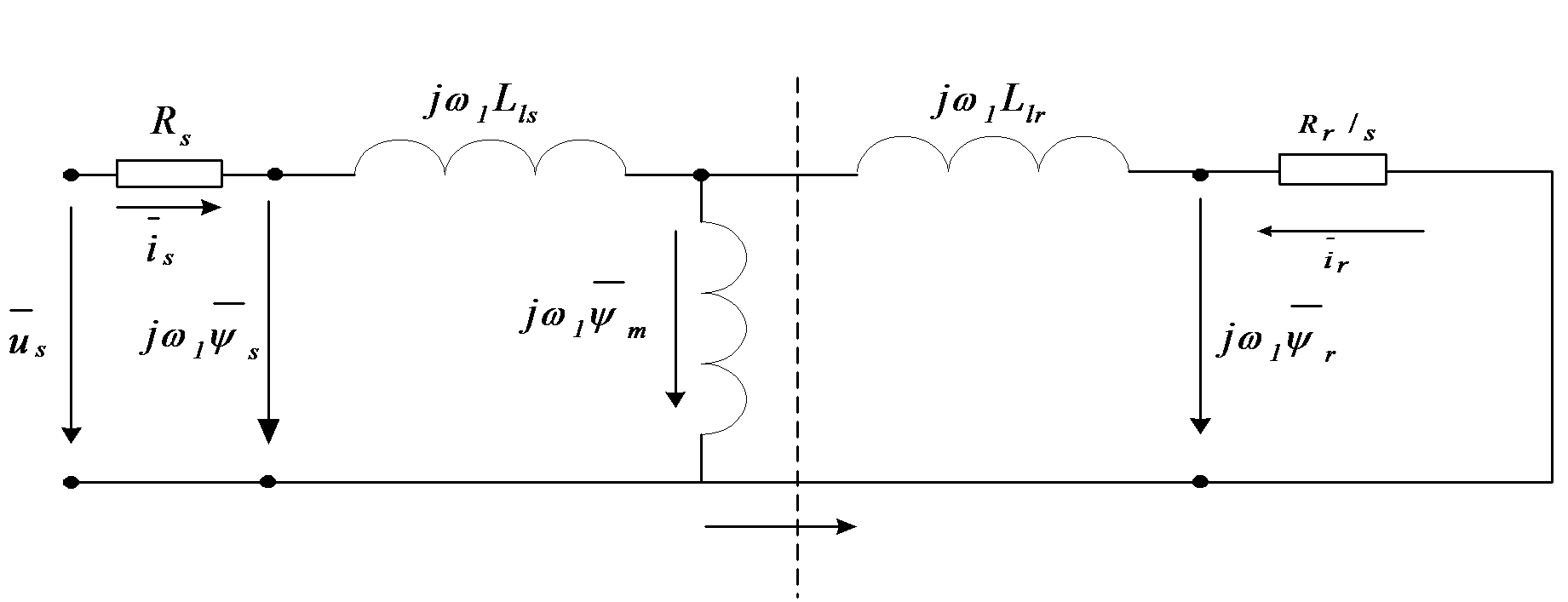
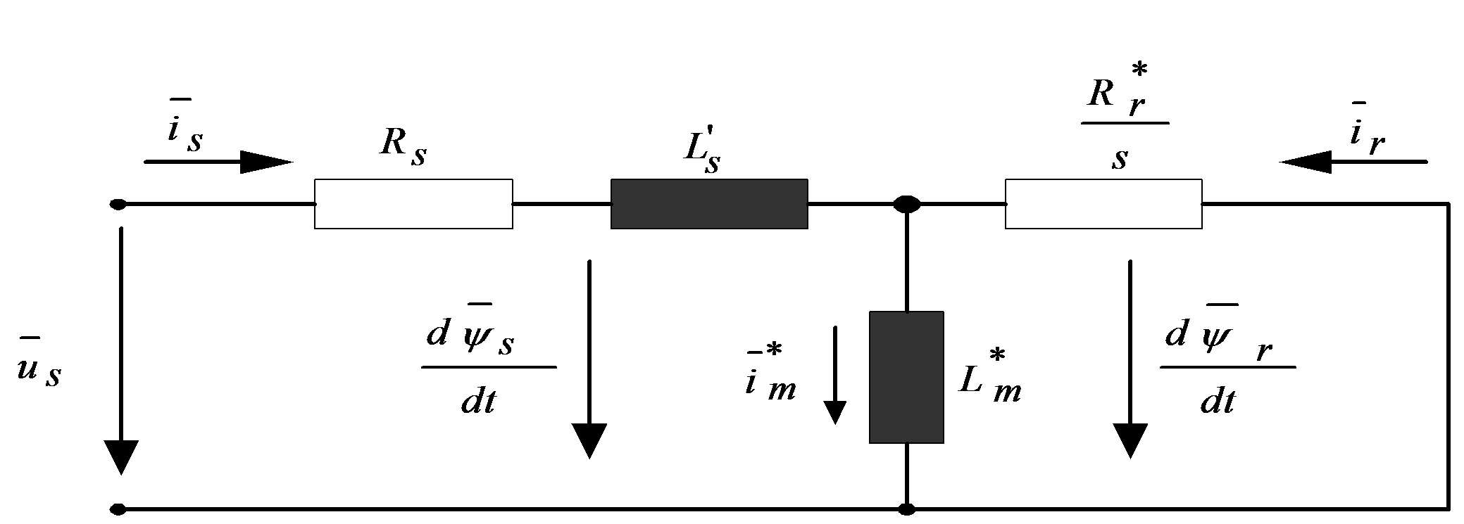
Equation (7.30) is nothing else but the equivalent circuit of the asynchronous motor in normal operation. The equivalent circuit of the asynchronous motor in this case is shown in Figure 1.7.

From the above statements it can be concluded that in normal operation, using a common reference frame, the machine equations become as simple as in the case of a transformator. For dynamic or transient analyses we use the equivalent circuits according to flux equations, instead of equivalent circuits according to voltage equations. Let us transform the flux equations now, using the equations ${\bar{i}}_{s} + {\bar{i}}_{r} = {\bar{i}}_{m}$ , and ${\bar{i}}_{m} \cdot L_{m} = {\bar{Ψ}}_{m}$ , where the first equation is that of vectorial magnetizing current, which is the result of the stator and rotor field induction, when 1:1 effective turn or reduction ratio is used, and the second is that of the equation of the flux of the main magnetic field. From equations (7.22) and (7.23) using and substituting the above statements we obtain the following flux equations:

Figure 7.7. Equivalent circuit of the AC motor in normal operation

${\bar{ψ}}_{s} = {\bar{i}}_{s} L_{s} + ({\bar{i}}_{m} - {\bar{i}}_{s}) L_{m} = {\bar{i}}_{s} (L_{s} - L_{m}) + {\bar{i}}_{m} L_{m} = {\bar{i}}_{m} L_{m} + {\bar{i}}_{s} L_{l s}$

(7.31)

${\bar{ψ}}_{r} = ({\bar{i}}_{m} - {\bar{i}}_{r}) L_{m} + {\bar{i}}_{r} L_{r} = {\bar{i}}_{m} L_{m} + {\bar{i}}_{r} (L_{r} - L_{m}) = {\bar{i}}_{m} L_{m} + {\bar{i}}_{r} L_{l r}$

(7.32)

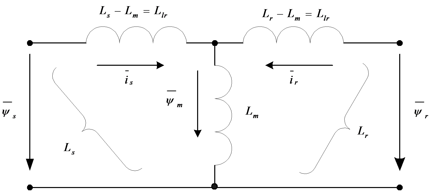
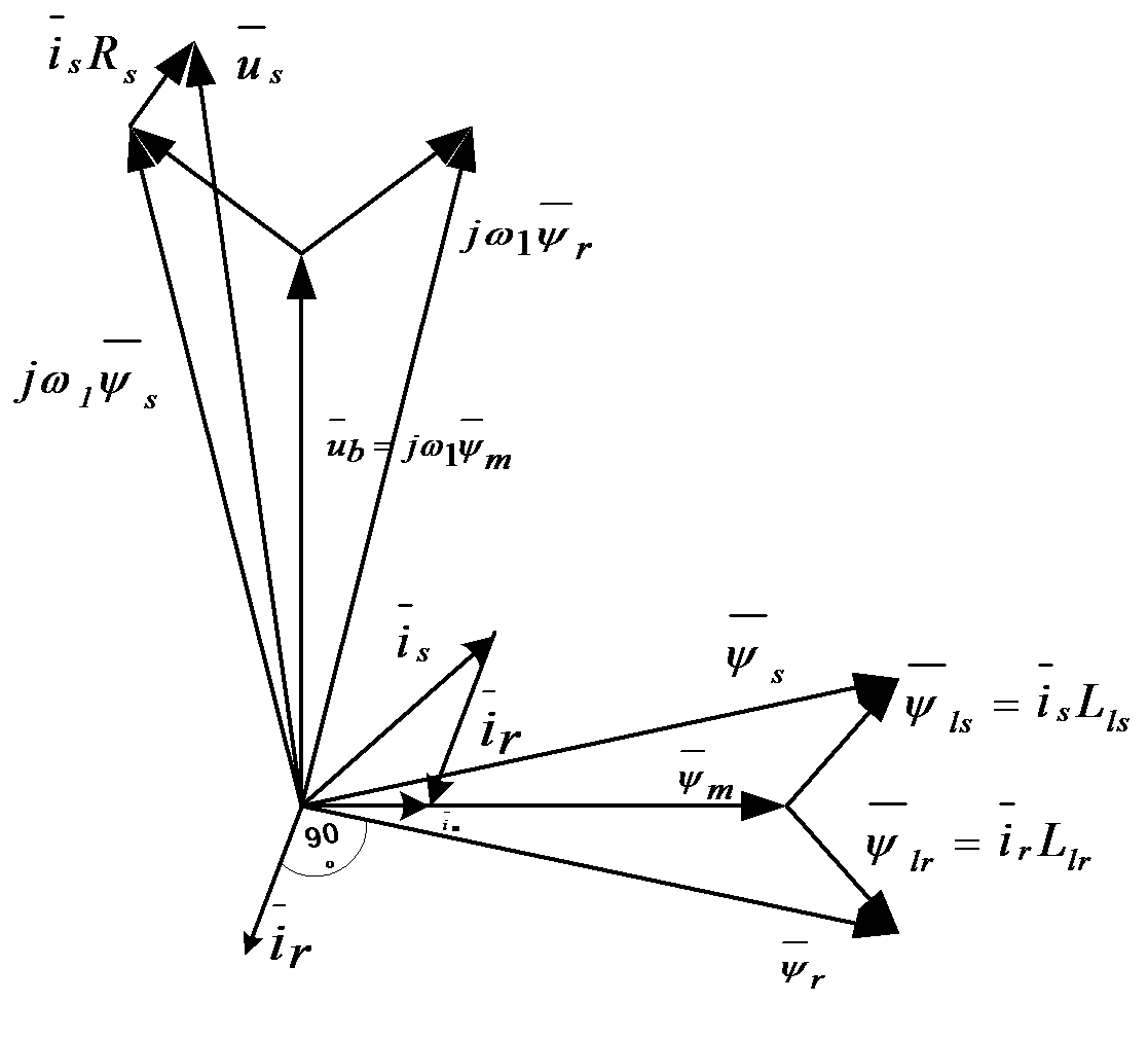
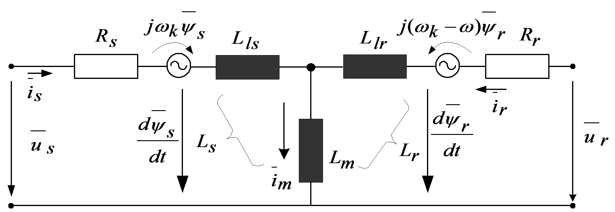
Based on the (7.31) and (7.32) equations the flux equivalent circuit is shown in Figure 7-8. The vectorial diagram of voltages and fluxes in a stationary case can be seen in Figure 7-9. According to the Figure 7-9, in synchronous speed co-ordinate system $ω_{k} = ω_{1}$ , all the vectors are constant, and the voltage and rotor equations become

${\bar{u}}_{s} = {\bar{i}}_{s} \cdot R_{s} + j ω_{1} {\bar{Ψ}}_{s}$ , (7.33)

$0 = \frac{\bar{u_{r}}}{s} = \bar{i_{r}} \cdot \frac{R_{r}}{s} + j ω_{1} \bar{Ψ_{r}}$

(7.34)

7.3. Modified Equivalent Circuits

The equivalent circuits stemming from the flux equations normally use a per unit effective turn or reduction ratio. In this case the magnitudes in relative units are $L_{m} \approx 2.5, L_{l s} \approx L_{l r} \approx 0.2$ . In many cases it is worth to choose a turn ratio which differs from the 1:1 ratio, because of the consistent simplifications in the motor equations. Let us introduce the fictive reduction factor a for the rotor quantities.

Figure 7.8. Equivalent circuit of fluxes

${\bar{Ψ}}_{r}^{*} = a \cdot {\bar{Ψ}}_{r}$ , ${\bar{i}}_{r}^{*} = \frac{{\bar{i}}_{r}}{a}$ , ${\bar{u}}_{r}^{*} = a \cdot {\bar{u}}_{r}^{*}$ , $R_{r}^{*} = a^{2} \cdot R_{r}$ . In this case the flux equations (7.31) and (7.32) will be

Figure 7.9. Vectorial diagram of fluxes and voltages

${\bar{ψ}}_{s} = {\bar{i}}_{m}^{*} L_{m}^{*} + {\bar{i}}_{s} L_{l s}^{*}$

(7.35)

${\bar{ψ}}_{r}^{*} = {\bar{i}}_{m}^{*} L_{m}^{*} + {\bar{i}}_{r}^{*} L_{l r}^{*}$

(7.36)

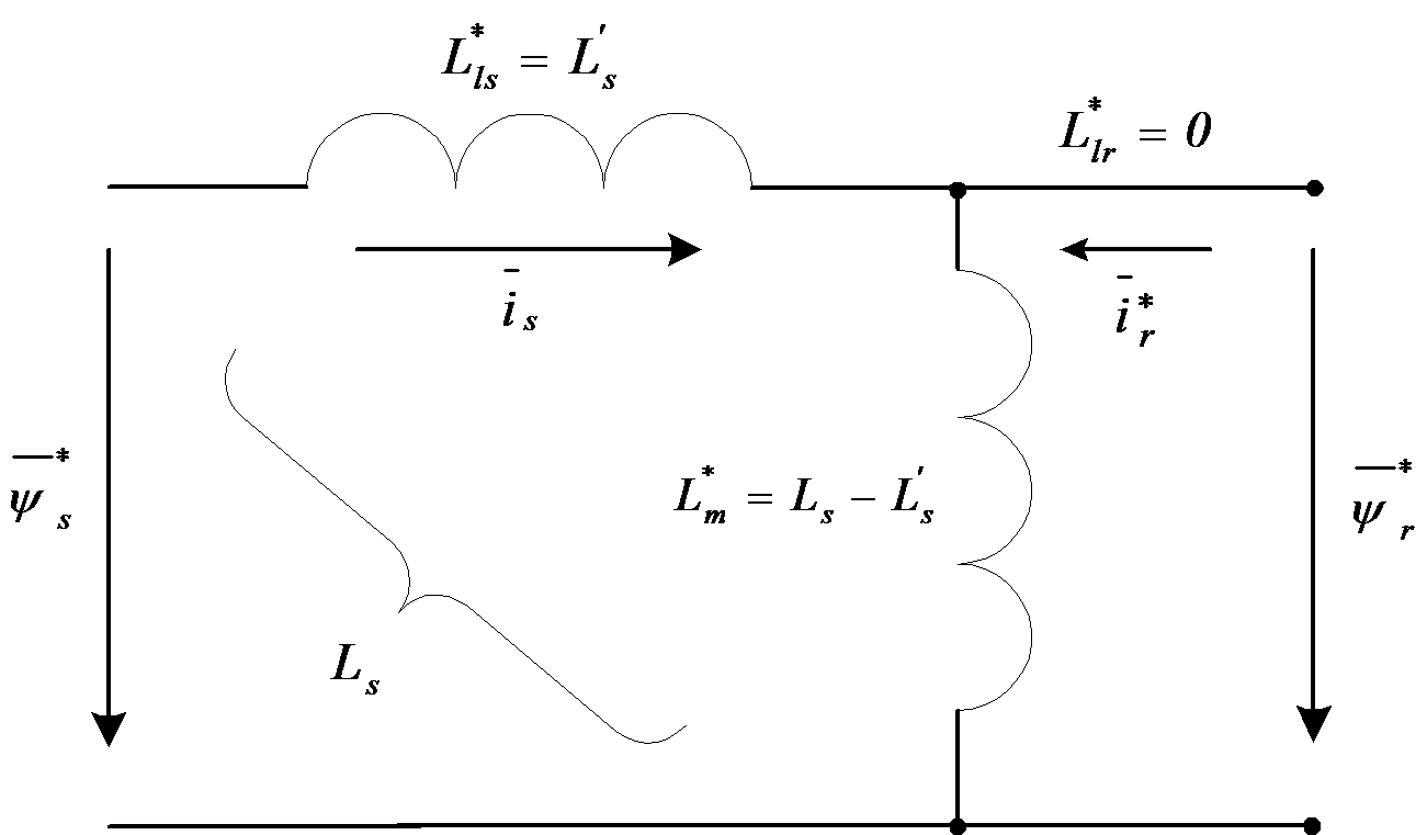
where $L_{m}^{*} = a \cdot L_{m}$ , $L_{r}^{*} = a^{2} \cdot L_{r}$ , $L_{l s}^{*} = L_{s} - L_{m}^{*}$ , $L_{l r}^{*} = L_{r}^{*} - L_{m}^{*}$ . The reduction factor can be chosen in such a way that, after reduction, one of the reduced leakage factors becomes zero. $L_{l r}^{*} = 0$ , if $L_{r}^{*} - L_{m}^{*} = a_{1}^{2} \cdot L_{r} - a_{1} \cdot L_{m} = 0$ , $a_{1} \cdot (a_{1} \cdot L_{r} - L_{m}) = 0$ $\Rightarrow$ $a_{1} = \frac{L_{m}}{L_{r}}$ and $L_{l s}^{*} = 0$ , if $L_{s} - L_{m}^{*} = L_{s} - a_{2} \cdot L_{m} = 0$ $\Rightarrow$ $a_{2} = \frac{L_{s}}{L_{m}}$ . If we use the above mentioned numbers for the inductance in the case of 1:1 reduction ratio, we get a1=2.5/2.5+0.11-0.4 and a2=2.5+0.1/2.51.04. Simplified flux equivalent circuits can be used in this case when the reduction ratio alters from 1:1, with a few percent. In Figure 710., and Figure 711. two simplified flux equivalent circuits are presented. Evaluating the fluxes marked by “*”,with the original inductance values (in the case of 1:1 reduction ratio), further simplification of the model is possible. There is obvious need to introduce the motor transient inductance ${L^{'}}_{s}$ , which is the resulting inductance from the primary site, neglecting the resistors and considering the secondary part in a short circuit. In the equivalent circuit (Figure 78.) according to fluxes, we can choose ${\bar{Ψ}}_{r} = 0$ instead of ${\bar{u}}_{r} = 0$ :

${L^{'}}_{s} = L_{l s} + \frac{L_{m} \cdot L_{l r}}{L_{m} + L_{l r}} \approx L_{l s} + L_{l r}$

(7.37)

${\bar{Ψ}}_{r} = 0 = L_{m} \cdot {\bar{i}}_{s} + L_{r} \cdot {\bar{i}}_{r}, {\bar{i}}_{r} = - \frac{L_{m}}{L_{r}} \cdot {\bar{i}}_{s}, {\bar{Ψ}}_{s} = L_{s} \cdot {\bar{i}}_{s} + L_{m} \cdot {\bar{i}}_{r}$

(7.38)

${L^{'}}_{s} = \frac{{\bar{Ψ}}_{s}}{{\bar{i}}_{s}} |_{{\bar{Ψ}}_{r} = 0} = L_{s} - \frac{L_{m}^{2}}{L_{r}} = (1 - \frac{L_{m}^{2}}{L_{s} \cdot L_{r}}) \cdot L_{s} = σ L_{s}$

(7.39)

Figure 7.10. Modified equivalent circuit with the elimination of stator leakage

$σ = \frac{{L^{'}}_{s}}{L_{s}} = 1 - \frac{L_{m}^{2}}{L_{s} \cdot L_{r}} = 1 - k$

(7.40)

Figure 7.11. Modified equivalent circuit for fluxes if the rotor leakage is eliminated

where is the resultant (total) leakage coefficient and k is the coupling coefficient. The ${L^{'}}_{r}$ rotor transient inductance is the secondary resultant inductance, neglecting the resistors and considering a short circuit in the primer circuit. So calculating with ${\bar{Ψ}}_{s} = 0$ we get

Figure 7.12. Equivalent circuit of the motor valid also for transient operation

$L' = L_{l s} + \frac{L_{m} \cdot L_{l r}}{L_{m} + L_{l r}} \approx L_{l s} + L_{l r}$

(7.41)

$L_{r}^{'} = \frac{\bar{Ψ_{r}}}{\bar{i_{r}}} |_{{\bar{Ψ}}_{s} = 0} = L_{r} - \frac{L_{m}^{2}}{L {}_{s}} = (1 - \frac{L_{m}^{2}}{L_{s} \cdot L_{r}}) \cdot L_{r} = σ L_{r}$

(7.42)

$σ = \frac{L_{r}^{'}}{L_{r}} = \frac{{L^{'}}_{s}}{L_{s}}$

(7.43)

In case of Figure 7-10., we have

$L_{m}^{*} = L_{s} - L^{'} {}_{s}= (1 - σ) \cdot L_{s}, L_{l s}^{*} = {L^{'}}_{s} = σ \cdot L_{s}$

(7.44)

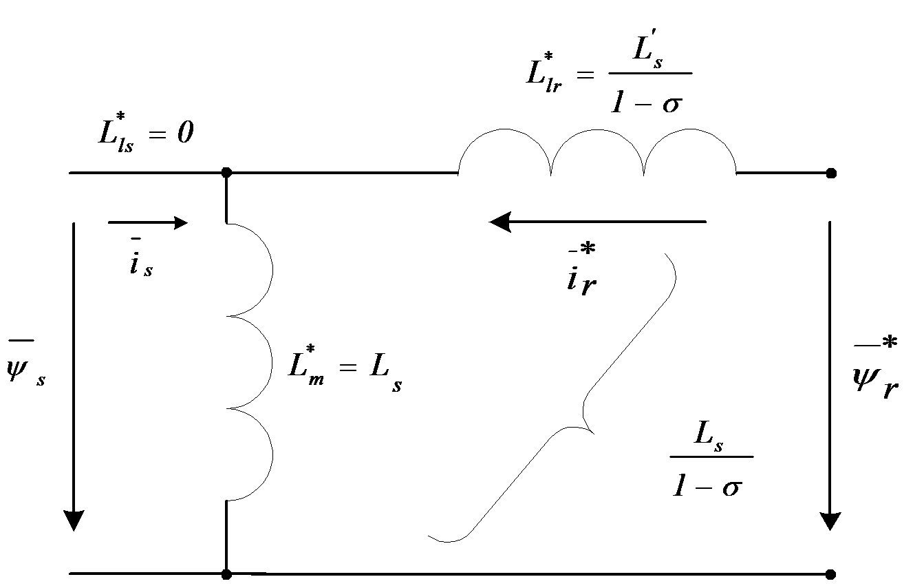
In case of Figure 7-11., we have

$L_{m}^{*} = L_{s}, L_{l r}^{*} = \frac{L_{s} \cdot {L^{'}}_{s}}{L_{s} - {L^{'}}_{s}} = \frac{{L^{'}}_{s}}{1 - σ}$

(7.45)

As it can be observed on the figures, the main field, in the case of the first figure, is ${\bar{Ψ}}_{m}^{*} = {\bar{Ψ}}_{r}^{*}$ , while, in the case of the second figure, it is ${\bar{Ψ}}_{m}^{*} = {\bar{Ψ}}_{s}$ . Knowing the values of $L_{s}$ , ${L^{'}}_{s}$ or $σ$ , both equivalent circuits of Figure 710. or Figure 711. can be useful. It is evident that in this case the reduction must be effectuated also for the voltage equations, as follows:

${\bar{u}}_{r} = {\bar{i}}_{r} \cdot R_{r} + \frac{d {\bar{Ψ}}_{r}}{d t} + j (ω_{k} - ω) \cdot {\bar{Ψ}}_{r}$

(7.46)

${\bar{u}}_{r}^{*} = {\bar{i}}_{r}^{*} \cdot R_{r}^{*} + \frac{d {\bar{Ψ}}_{r}^{*}}{d t} + j (ω_{k} - ω) \cdot {\bar{Ψ}}_{r}^{*}$

(7.47)

This form matches the original equation, so if we choose the mode of reduction the “*” notation can be omitted. The Figure 7-12. presents the motor equivalent circuit, which is also valid for transient operation of the machines.

Taking the above statements into consideration, and regarding the modified equivalent circuits, for the purpose of further analysis, an equivalent circuit has been chosen, where the rotor leakage impedance has been included into the expression of the stator transient impedance. The new equivalent circuit can be seen in Figure 7-13. In this case, as we will see later on, the program calculates the voltages corresponding to the necessary current of the motor, instead of using a current control loop. Because the algorithm running time is less than the rotor time constant, the flux can be considered as constant. Consequently, the chosen equivalent circuit, where the rotor leakage impedance is properly included in the stator transient impedance (Ls'), is a good choice.

Figure 7.13. The chosen equivalent circuit

After reducing the motor's physical parameters and transforming the equations mathematically, the expression of the stator voltage vector equation will be as follows:

${\bar{u}}_{s} = {\bar{i}}_{s} R_{s} + \frac{d {\bar{i}}_{s} L_{s}'}{d t} + j ω_{1} {\bar{i}}_{s d} L_{_{m}}^{}$

(7.48)

As we can see on the following pages, this equation will play a very important role in setting up the control structures, and also in applications.

7.4. Setting up the Model

Let us choose first a standstill co-ordinate system $ω_{k} = 0$ , which means that the common co-ordinate system is a stationary one. Replacing the value $ω_{k} = 0$ in the general equations of the motor given by (7.20), (7.21), (7.22), and (7.23), the following vectorial voltage equations conclude:

${\bar{u}}_{s} = {\bar{i}}_{s} \cdot R_{s} + \frac{d {\bar{Ψ}}_{s}}{d t}$

(7.49)

$\bar{u_{r}} = \bar{i_{r}} \cdot R_{r} + \frac{d \bar{Ψ_{r}}}{d t} - j ω \cdot \bar{Ψ_{r}} = 0$

(7.50)

Let us fix ${\bar{Ψ}}_{r}$ and ${\bar{i}}_{s}$ as state variables. After the elimination of the terms ${\bar{i}}_{r}$ and ${\bar{Ψ}}_{s}$ from the above differential equation system, we get the following equations:

${\bar{Ψ}}_{s} = \frac{L_{m}}{L_{r}} \cdot {\bar{Ψ}}_{r} + (L_{s} - \frac{L_{m}^{2}}{L_{r}}) \cdot {\bar{i}}_{s} = \frac{L_{m}}{L_{r}} \cdot {\bar{Ψ}}_{r} + L_{s} \cdot (1 - \frac{L_{m}^{2}}{L_{s} \cdot L_{r}}) \cdot {\bar{i}}_{s} = \frac{L_{m}}{L_{r}} \cdot {\bar{Ψ}}_{r} + L_{s} \cdot σ \cdot {\bar{i}}_{s}$

(7.51)

${\bar{u}}_{s} = R_{s} \cdot {\bar{i}}_{s} + \frac{d {\bar{Ψ}}_{s}}{d t} = R_{s} \cdot {\bar{i}}_{s} + \frac{d (\frac{L_{m}}{L_{r}} \cdot \bar{Ψ_{r}} + L_{s} \cdot σ \cdot {\bar{i}}_{s})}{d t} = R_{s} \cdot {\bar{i}}_{s} + \frac{L_{m}}{L_{r}} \cdot \frac{d {\bar{Ψ}}_{r}}{d t} + L_{s} \cdot σ \cdot \frac{d {\bar{i}}_{s}}{d t}$

(7.52)

${\bar{u}}_{r} = R_{r} \cdot {\bar{i}}_{r} + \frac{d {\bar{Ψ}}_{r}}{d t} - j ω \cdot {\bar{Ψ}}_{r} = \frac{R_{r}}{L_{r}} \cdot {\bar{Ψ}}_{r} - \frac{L_{m} \cdot R_{r}}{L_{r}} \cdot {\bar{i}}_{s} + \frac{d {\bar{Ψ}}_{r}}{d t} - j ω \cdot {\bar{Ψ}}_{r} = 0$

(7.53)

Solving the above equations according to the chosen state variables we get

$\frac{d {\bar{Ψ}}_{r}}{d t} = (j ω - \frac{R_{r}}{L_{r}}) \cdot {\bar{Ψ}}_{r} + \frac{L_{m} R_{r}}{L_{r}} \cdot {\bar{i}}_{s}$

(7.54)

$\frac{d {\bar{i}}_{s}}{d t} = \frac{1}{L_{s} \cdot σ} [- R_{s} \cdot {\bar{i}}_{s} - \frac{L_{m}^{2} \cdot R_{r}}{L_{r}^{2}} \cdot {\bar{i}}_{s} - \frac{L_{m}}{L_{r}} (j ω - \frac{R_{r}}{L_{r}}) \cdot {\bar{Ψ}}_{r}] + \frac{1}{L \cdot σ} \cdot {\bar{u}}_{s}$

(7.55)

For simplifying the above equations let us make the notation.

$- (R_{s} + \frac{L_{m}^{2} \cdot R_{r}}{L_{r}^{2}}) = - \bar{R}$

(7.56)

The has been defined in (7.40). Using again the complex representation of the vectors $\bar{Ψ_{r}} = Ψ_{r d} + j Ψ_{r q}$ and ${\bar{i}}_{s} = i_{s}_{d} + i_{s}_{q}, {\bar{u}}_{s} = u_{s}_{d} + j \cdot u_{s}_{q}$ , the model of the induction motor when ${\bar{Ψ}}_{r}, {\bar{i}}_{s}$ are considered as state variables can be written in the following matrix form:

$\frac{d}{d t} [\begin{matrix} i_{s}_{d} \\ i_{s}_{q} \\ ψ_{r d} \\ ψ_{r q} \end{matrix}] = [\begin{matrix} - \frac{\bar{R}}{L_{s} σ} & 0 & \frac{L_{m} R_{r}}{L_{s} σ L_{r}^{2}} & \frac{L_{m} ω}{L_{s} σ L_{r}} \\ 0 & - \frac{\bar{R}}{L_{s} σ} & - \frac{L_{m} ω}{L_{s} σ L_{r}} & \frac{L_{m} R_{r}}{L_{s} σ L_{r}^{2}} \\ \frac{L_{m} R_{r}}{L_{r}} & 0 & - \frac{R_{r}}{L_{r}} & - ω \\ 0 & \frac{L_{m} R_{r}}{L_{r}} & ω & - \frac{R_{r}}{L_{r}} \end{matrix}] • [\begin{matrix} i_{s}_{d} \\ i_{s}_{q} \\ ψ_{r d} \\ ψ_{r q} \end{matrix}] + [\begin{matrix} \frac{1}{L σ} & 0 \\ 0 & \frac{1}{L σ} \\ 0 & 0 \\ 0 & 0 \end{matrix}] • [\begin{matrix} u_{s}_{d} \\ u_{s}_{q} \end{matrix}]$

(7.57)

In same references when the two phase coordinate system does not rotate the quantities $u_{s α}, u_{s β}, i_{s α}, i_{s β}, ψ_{s α}, ψ_{s β},$ are used instead of d,q quantities. So in the rest of the theses the when , components are used these refer to a stationary two phase coordinate system, when d,q components are used these will be the quantities in a special rotating two phase-system (field coordinates). The model of the induction motor will be described in field co-ordinates (in none of these models of the Asynchronous Motor do we take the mechanical losses into account), considering now the motion or cinematic equation of the motor, which is very important when we apply stochastic observers for the motor. As a basis, now again, the equations deduced in the previous paragraph, but with notations slightly changed as described also in [14], [15] will be used. This system of equations is nonlinear. The indices "r" and "s" mean rotor and stator, respectively:

${\bar{u}}_{s} (t) = R_{s} {\bar{i}}_{s} (t) + \frac{d {\bar{ψ}}_{s} (t)}{d t} = R_{s} {\bar{i}}_{s} (t) + L_{s} \frac{d}{d t} {\bar{i}}_{s} (t) + L_{m} \frac{d}{d t} ({\bar{i}}_{r} (t) e^{i ε (t)})$

(7.58)

$0 = R_{r} {\bar{i}}_{r} (t) + \frac{d}{d t} {\bar{ψ}}_{r} (t) = R_{r} {\bar{i}}_{r} (t) + L_{r} \frac{d}{d t} {\bar{i}}_{r} (t) + L_{m} \frac{d}{d t} {\bar{i}}_{s} (t) e^{- j ε (t)}$

(7.59)

$m_{e} (t) = \frac{2}{3} p L_{m} I_{m} {{\bar{i}}_{s} (t) {[{\bar{i}}_{r} (t) e^{j ε (t)}]}^{*}}$

(7.60)

$\frac{d ω (t)}{d t} = \frac{P}{J} (m_{e} (t) - m_{L} (t)),$ , where $\frac{d ε (t)}{d t} = ω (t)$ is the rotor angular velocity.(7.61)

The definition of the inductances in these equations and the total leakage factor is as follows:

$L_{s} = L_{l s} + L_{m} = (1 + σ_{s}) L_{m}, L_{r} = L_{l r} + L_{m} = (1 + σ_{r}) L_{m}, σ = 1 - \frac{1}{(1 + σ_{s}) (1 + σ_{{}_{r}})}$

(7.62)

where Lm is the main inductance of the motor, $R_{s}$ and $R_{r}$ are the resistances of the windings and Lls, Llr , are the leakage inductances of the stator and rotor respectively.

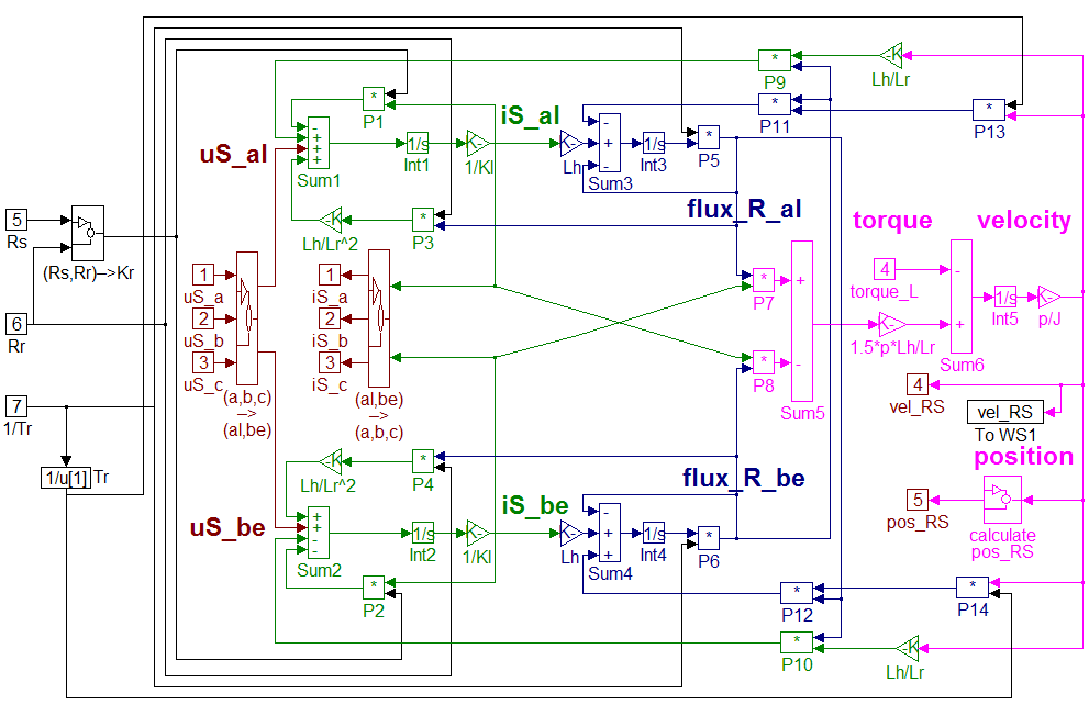
This model has been realized in SIMULINK for test and simulation purposes. See Figure 7-15. for the graphic realization. We will now define the model of the asynchronous motor in field co-ordinates. This will make it possible to implement the controller in field co-ordinates. Field orientation is described in detail in [16], and in the following sections. The basic principle is that we convert all values to the co-ordinate system of the magnetic field, decompose the stator current vector into a field generating and a torque generating ( $i_{s d}$ and $i_{s q}$ ) component. At this moment the actual control becomes very simple. Since the program is designed so that the field weakening range will not be reached, the field generating component of the stator current voltage vector can be kept at a constant value to generate a necessary field, and control the torque generating component according to the speed. This means that the output of the speed controller is the reference for $i_{s q}$ . We will eliminate the use of flux in the model, and we will use the magnetizing current instead. The connection between these two variables is the following:

${\bar{i}}_{m r} = (1 + σ_{r}) {\bar{i}}_{r} (t) e^{j ε (t)} + {\bar{i}}_{s} (t) = {\bar{i}}_{m r} e^{j ρ (t)} = \frac{1}{L_{m}} {\bar{ψ}}_{r} (t) e^{_{j ε (t)}}$

(7.63)

where is the angle of the rotor magnetizing current vector with respect of the stationary axis. This quantity will play an important role in vector control when the special reference frame will be fixed to the rotor flux. The transformation between the systems will be done by the following transformation:

${\bar{u}}_{s} e^{- j ρ} = u_{s d} + j u_{s q}, {\bar{i}}_{s} e^{- j ρ} = i_{s d} + j i_{s q}$

(7.64)

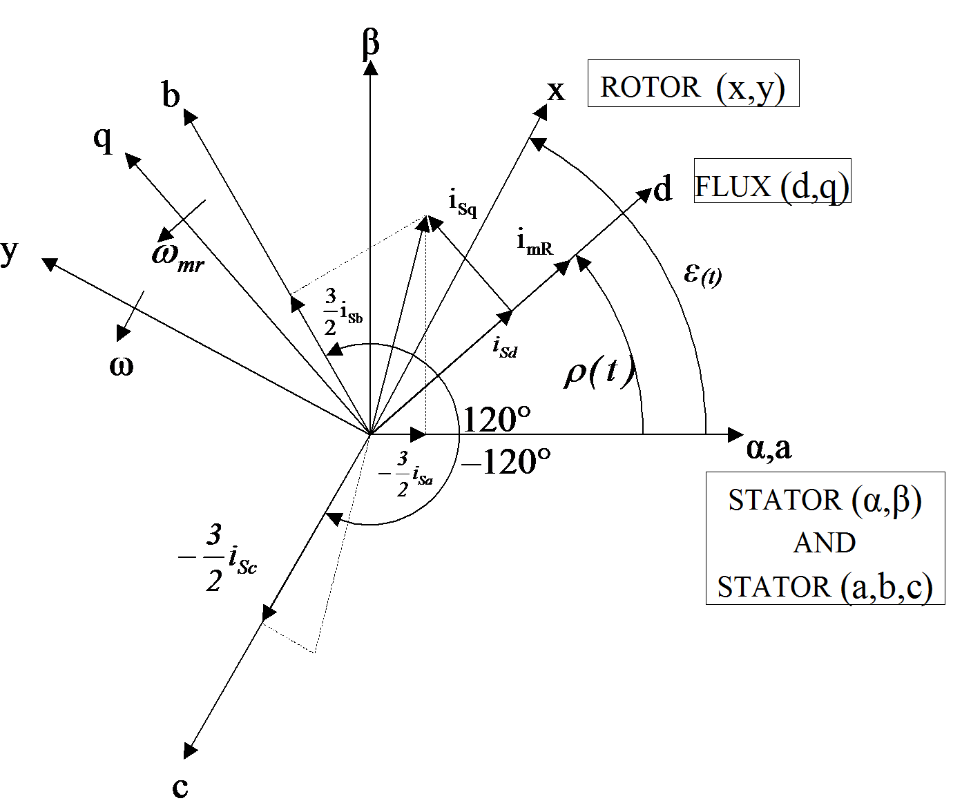
First, let us consider a brief overview of the state vectors (also called state phasors) represented in different co-ordinate systems as shown in Figure 7-14.

7.5. Stator Coordinates

Let us now switch to a Descartes coordinate system and fix it to the stator (, stationary reference frame). In this case the speed of the rotating coordinate system is $ω_{k} = 0$ . Let us choose the stator current and the rotor flux to be the state variables. It means that we have to express these quantities from the general motor model described in equations (7.20)-(7.23). The resulted scalar model-equations are:

$u_{s α} (t) = (R_{s} + \frac{L_{s} (1 - σ)}{T_{r}}) i_{s α} (t) + σ L_{s} \frac{d}{d t} i_{s α} (t) - \frac{L_{m}}{L_{r} \cdot T_{r}} Ψ_{r α} (t) - \frac{L_{m}}{L_{r}} ω (t) Ψ_{r β} (t)$

(7.65)

$u_{s β} (t) = (R_{s} + \frac{L_{s} (1 - σ)}{T_{r}}) i_{s β} (t) + σ L_{s} \frac{d}{d t} i_{s β} (t) + \frac{L_{m}}{L_{r}} ω (t) Ψ_{r α} (t) - \frac{L_{m}}{L_{r} \cdot T_{r}} Ψ_{r β} (t)$

(7.66)

$Ψ_{r α} (t) = L_{m} i_{s α} (t) - T_{r} \frac{d}{d t} Ψ_{r α} (t) - T_{r} ω (t) Ψ_{r β} (t)$

(7.67)

$Ψ_{r β} (t) = L_{m} i_{s β} (t) + T_{r} ω (t) Ψ_{r α} (t) - T_{r} \frac{d}{d t} Ψ_{r β} (t)$

(7.68)

The rotor time constant is denoted by $T_{r} = \frac{L_{r}}{R_{r}}$ .

These equations are now rewritten in a state space form with state variables isα, isβ, Ψrα and Ψrβ.

$\frac{d}{d t} [\begin{matrix} i_{s α} \\ i_{s β} \\ Ψ_{r α} \\ Ψ_{r β} \end{matrix}] = [\begin{matrix} a_{11} & 0 & a_{12} & - a_{13} \\ 0 & a_{11} & a_{13} & a_{12} \\ a_{21} & 0 & a_{22} & - a_{23} \\ 0 & a_{21} & a_{23} & a_{22} \end{matrix}] [\begin{matrix} i_{s α} \\ i_{s β} \\ Ψ_{r α} \\ Ψ_{r β} \end{matrix}] + [\begin{matrix} b & 0 \\ 0 & b \\ 0 & 0 \\ 0 & 0 \end{matrix}] [\begin{matrix} u_{s α} \\ u_{s β} \end{matrix}]$

(7.69)

$a_{11} = - (\frac{1}{σ T_{s}} + \frac{1 - σ}{σ} \cdot \frac{1}{T_{r}}); a_{12} = \frac{L_{m}}{σ L_{s} L_{r}} \cdot \frac{1}{T_{r}}; a_{13} = - \frac{L_{m}}{σ L_{s} L_{r}} \cdot ω$

(7.70)

$a_{21} = \frac{L_{s}}{T_{r}}; a_{22} = - \frac{1}{T_{r}}; a_{23} = ω$

(7.71)

$b = \frac{1}{σ L_{s}}$

(7.72)

Figure 7.14. Connection between different coordinate systems

The stator time constant is denoted by $T_{s} = \frac{L_{s}}{R_{s}}$ . The kinematic equations of the motor in stator coordinates are as follows:

$m_{e} = \frac{2}{3} p \frac{L_{m}}{L_{r}} (i_{s β} (t) Ψ_{r α} (t) - i_{s α} (t) Ψ_{r β} (t))$

(7.73)

$\frac{d}{d t} ω (t) = \frac{p}{J} (m_{e} (t) - m_{L} (t))$

(7.74)

$\frac{d}{d t} ε (t) = ω (t)$

(7.75)

where mL is the mechanical torque and p is the magnetic pole count.

7.6. Field Coordinates

Choosing the rotor flux as orientation quantity, that means all quantities are viewed from the rotor flux point of view, which are usually called field coordinates. The advantage of using this reference frame is that all quantities are constant in the steady state. The flux is now eliminated by introducing a new quantity called magnetizing current (rotor current cannot be measured) see eq. (7.63). The stator current (in field coordinates) and the magnetizing current are now chosen to be the state variables. The resulted scalar model-equations are:

$u_{s d} (t) = R_{s} i_{s d} (t) + σ L_{s} \frac{d}{d t} i_{s d} (t) - σ L_{s} ω_{1} (t) i_{s q} (t) + (1 - σ) L_{s} \frac{d}{d t} i_{m r} (t)$

(7.76)

$u_{s q} (t) = R_{s} i_{s q} (t) + σ L_{s} \frac{d}{d t} i_{s q} (t) + σ L_{s} ω_{1} (t) i_{s d} (t) + (1 - σ) L_{s} ω_{1} (t) i_{m r} (t)$

(7.77)

$i_{s d} (t) = i_{m r} (t) + T_{r} \frac{d}{d t} i_{m r} (t)$

(7.78)

$i_{s q} (t) = (ω_{m r} (t) - ω (t)) T_{r} i_{m r} (t)$

(7.79)

Let us now rewrite these equations in a state space form where state variables iSd, iSq and imR are used. Notice that by introducing the magnetizing current we need only three state variables.

$\frac{d}{d t} [\begin{matrix} i_{s d} \\ i_{m r} \\ i_{s q} \end{matrix}] = [\begin{matrix} - \frac{1}{σ} \frac{1}{T_{s}} & - \frac{1 - σ}{σ} & ω_{m r} \\ \frac{1}{T_{r}} & - \frac{1}{T_{r}} & 0 \\ - ω_{m r} & - \frac{1 - σ}{σ} ω_{m r} & - \frac{1}{σ} \frac{1}{T_{s}} \end{matrix}] [\begin{matrix} i_{s d} \\ i_{m r} \\ i_{s q} \end{matrix}] + \frac{1}{σ T_{s} R_{s}} [\begin{matrix} u_{s d} \\ u_{s q} \end{matrix}]$

(7.80)

Where $ω_{m r} = ω + ω_{s l i p}$ , that is, the flux speed equals to the rotor speed plus the slip angular velocity of the rotor flux. The kinematic equations of the motor in field coordinates are:

$m_{e} (t) = \frac{2}{3} p (1 - σ) L_{s} i_{m r} (t) i_{s q} (t)$

(7.81)

The forms of equations remains unchanged in this coordinate system too. Equations presents the transformation matrices between the three-phase and the Descartes stationary coordinate systems, describes the connection between the stator and the field coordinates.

$[\begin{matrix} q_{α} \\ q_{β} \end{matrix}] = [\begin{matrix} \frac{2}{3} & - \frac{1}{3} & - \frac{1}{3} \\ 0 & \frac{1}{\sqrt{3}} & - \frac{1}{\sqrt{3}} \end{matrix}] [\begin{matrix} q_{a} \\ q_{b} \\ q_{c} \end{matrix}]; [\begin{matrix} q_{a} \\ q_{b} \\ q_{c} \end{matrix}] = [\begin{matrix} 1 & 0 \\ - \frac{1}{2} & \frac{\sqrt{3}}{2} \\ - \frac{1}{2} & - \frac{\sqrt{3}}{2} \end{matrix}] [\begin{matrix} q_{α} \\ q_{β} \end{matrix}]$

(7.82)

$[\begin{matrix} q_{s d} \\ q_{s q} \end{matrix}] = [\begin{matrix} \cos ε & \sin ε \\ - \sin ε & \cos ε \end{matrix}] [\begin{matrix} q_{s α} \\ q_{s β} \end{matrix}]; [\begin{matrix} q_{s α} \\ q_{s β} \end{matrix}] = [\begin{matrix} \cos ε & - \sin ε \\ \sin ε & \cos ε \end{matrix}] [\begin{matrix} q_{s d} \\ q_{s q} \end{matrix}]$

(7.83)

Figure 7-14. is a summary of the state vectors (also called state phasors) represented in different coordinate systems. Note that the rotor based variables are completely eliminated.

7.7. Model assumptions for the FOC method

Using the field oriented model of the motor, it has theoretically become possible to realize a control in field orientation, which makes it extremely easy to control speed by controlling $i_{s q}$ . However, our system of equations is nonlinear. We will eliminate this non-linearity by decoupling the nonlinear terms. This method has been described in [14], and detailed treatment is also given in [17]:

7.7.1. Decoupling of the Nonlinearity

We can see from (7.63), - that the model of the induction motor is nonlinear and time-variant. Let us now examine how nonlinearity is eliminated by decoupling the undesirable nonlinear and coupling terms.

$u_{s d} = u_{s d}^{L i n} + u_{s d}^{C o u p l e} = [R_{s} i_{s d} + σ L_{s} \frac{d}{d t} i_{s d}] + [- σ L_{s} ω_{1} i_{s q} + (1 - σ) L_{s} \frac{d}{d t} i_{m r}]$

(7.84)

$u_{s q} = u_{s q}^{L i n} + u_{s q}^{C o u p l e} = [R_{s} i_{s q} + σ L_{s} \frac{d}{d t} i_{s q}] + [σ L_{s} ω_{1} i_{s d} + (1 - σ) L_{s} ω_{s} i_{m r}]$

(7.85)

$u_{s d}^{L i n} = u_{s d} - u_{s d}^{C o u p l e} = [R_{s} i_{s d} + σ L_{s} \frac{d}{d t} i_{s d}]$

(7.86)

$u_{s q}^{L i n} = u_{s q} - u_{s q}^{C o u p l e} = [R_{s} i_{s q} + σ L_{s} \frac{d}{d t} i_{s q}]$

(7.87)

We would like to control the speed. Let us recall . The torque is directly proportional to imr and to isq. Because Tr is large, imr cannot be used for a quick control. The leakage factor of iSq is small, that is why iSq can be used to control the torque and the speed. We get the best dynamic behaviour when imr is kept constant, therefore $\frac{d}{d t} i_{m r} = 0$ can be assumed. This will remove the last non-linearity by making $K_{J}$ constant: Supposing that the main inductance Lm is time invariant, the rotor flux Ψr is kept constant, too. Under this assumption, using , , , and -(7.87) we get the following linear and decoupled model of the induction motor:

$\frac{d}{d t} [\begin{matrix} i_{s d} \\ i_{m r} \\ i_{s q} \\ ω \\ ε \end{matrix}] = [\begin{matrix} - \frac{1}{σ T_{s}} & 0 & 0 & 0 & 0 \\ \frac{1}{T_{r}} & - \frac{1}{T_{r}} & 0 & 0 & 0 \\ 0 & 0 & - \frac{1}{σ T_{s}} & 0 & 0 \\ 0 & 0 & K_{J} & 0 & 0 \\ 0 & 0 & 0 & 1 & 0 \end{matrix}] [\begin{matrix} i_{s d} \\ i_{m r} \\ i_{s q} \\ ω \\ ε \end{matrix}] + [\begin{matrix} \frac{1}{σ L_{s}} & 0 & 0 \\ 0 & 0 & 0 \\ 0 & \frac{1}{σ L_{s}} & 0 \\ 0 & 0 & - \frac{p}{J} \\ 0 & 0 & 0 \end{matrix}] [\begin{matrix} u_{s d}^{L i n} \\ u_{s q}^{L i n} \\ m_{L} \end{matrix}]$

(7.88)

Where

$K_{J} = \frac{2}{3} \frac{p^{2}}{J} (1 - σ) L_{s} i_{m r}^{r e f} = \frac{2}{3} \frac{p^{2}}{J} (1 - σ) L_{s} \frac{Ψ_{r}^{r e f}}{L_{m}} = c o n s t$

(7.89)

Assuming that $i_{m r}^{r e f} = \frac{Ψ_{r}^{r e f}}{L_{m}}$ is kept constant, KJ is also constant. In this case the system described by can be split into two independent parts, the direct (denoted by d) and the quadrature (denoted by q) subsystem:

$\frac{d}{d t} [\begin{matrix} i_{s d} \\ i_{m r} \end{matrix}] = [\begin{matrix} - \frac{1}{σ T_{s}} & 0 \\ \frac{1}{T_{r}} & - \frac{1}{T_{r}} \end{matrix}] [\begin{matrix} i_{s d} \\ i_{m r} \end{matrix}] + [\begin{matrix} \frac{1}{σ L_{s}} \\ 0 \end{matrix}] u_{s d}^{L i n}, y_{d} = [\begin{matrix} 0 & 1 \end{matrix}] [\begin{matrix} i_{s d} \\ i_{m r} \end{matrix}]$

(7.90)

$\frac{d}{d t} [\begin{matrix} i_{s q} \\ ω \\ ε \end{matrix}] = [\begin{matrix} - \frac{1}{σ T_{s}} & 0 & 0 \\ K_{J} & 0 & 0 \\ 0 & 1 & 0 \end{matrix}] [\begin{matrix} i_{s q} \\ ω \\ ε \end{matrix}] + [\begin{matrix} \frac{1}{σ L_{s}} & 0 \\ 0 & - \frac{p}{J} \\ 0 & 0 \end{matrix}] [\begin{matrix} u_{s q}^{L i n} \\ m_{L} \end{matrix}], y_{q} = [\begin{matrix} 0 & 1 & 0 \end{matrix}] [\begin{matrix} i_{s q} \\ ω \\ ε \end{matrix}]$

(7.91)

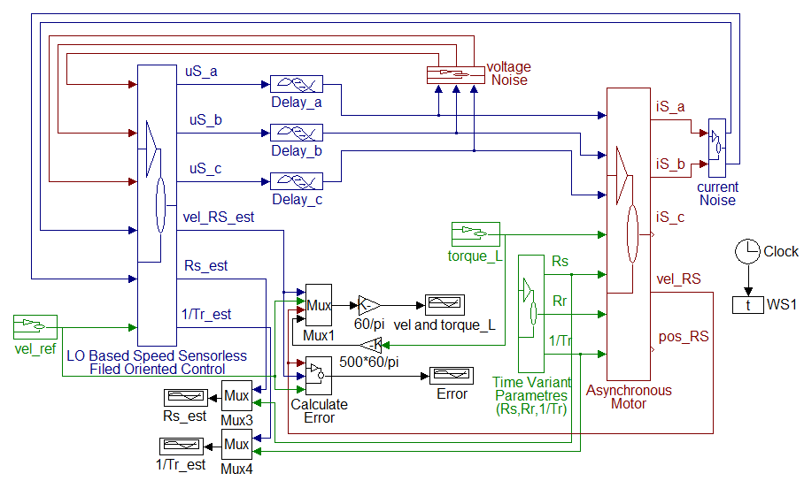
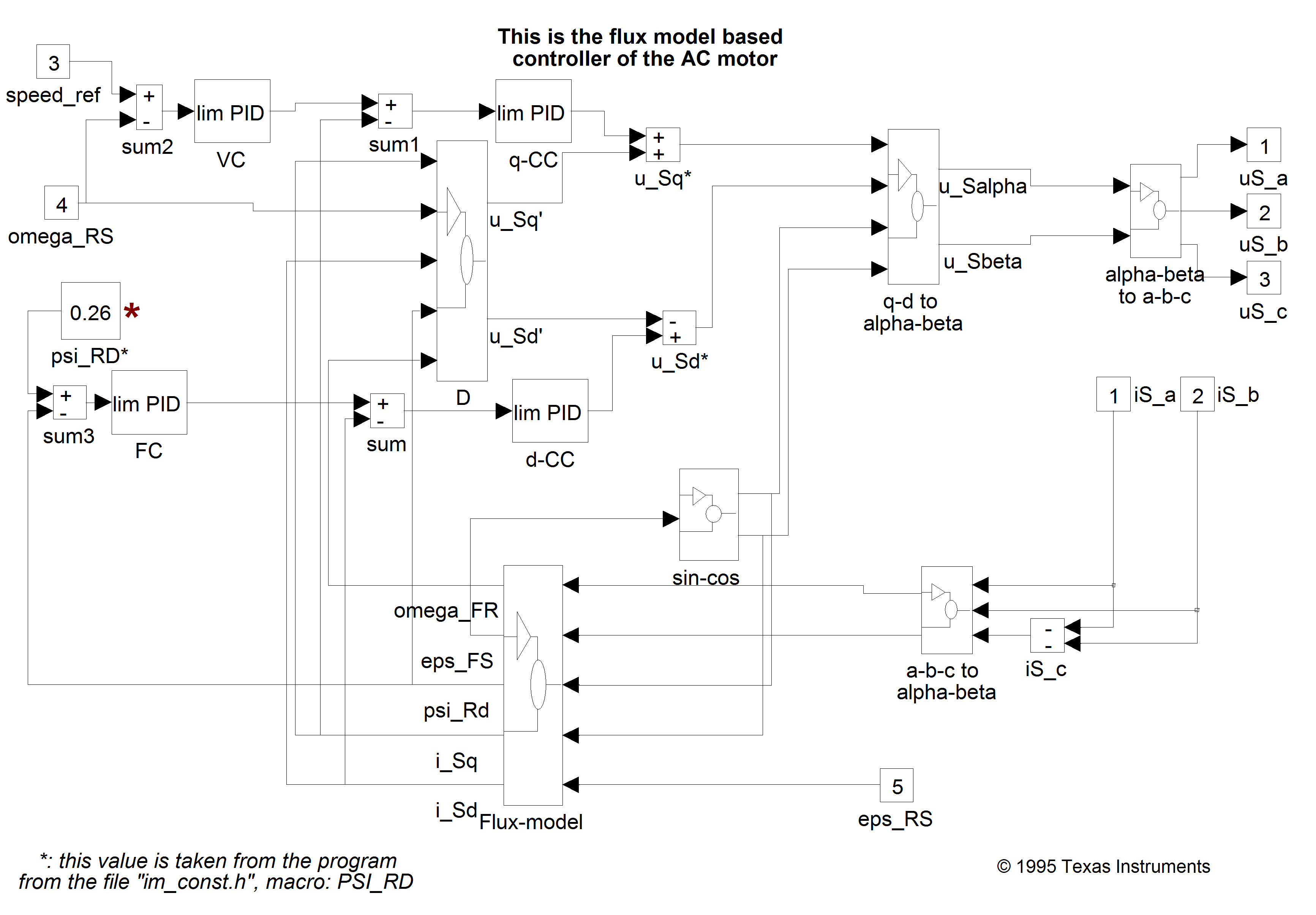
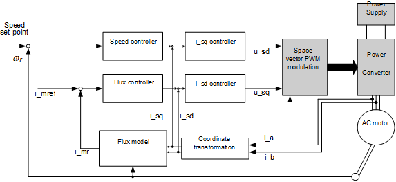
After this it is possible to control the motor, provided that we are able to convert all values to field co-ordinates. This is made by the flux model (see the description later in the Simulink realization in Figure 7-21. and Figure 7-22.). The form of the flux model which has been realized here is based on [16], [18] and a Simulink realization done by dSPACE GmbH. After realizing the flux model control becomes possible. The first loop of the control is a controller for imr, which is in fact a controller for the rotor flux. There is a controller for isd, which will force the correct imr. The second loop begins with a controller for $ω$ , followed by a controller for isq, which will force the correct torque, and implicitly will realize the correct velocity. The overall control structure is shown in Figure 7-23. and Figure 7-24.

7.7.2. The Matlab/Simulink Model of the AC Motor

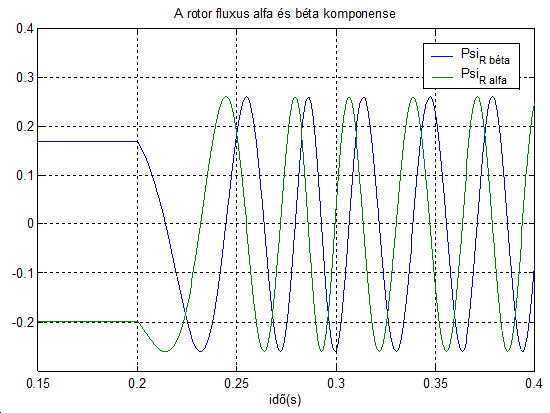
The model of the AC motor, which is sometimes called simply ASM = Asynchronous Motor, has been implemented in Simulink according to the equations as described in [16] and [14]. The actual model of the ASM can be seen in Figure 7-15. This model is based on the mathematical model described in [16]. However, it has been adapted to the requirements of Simulink. For the sake of simplicity, all vector variables have been substituted by scalar variables. The model is in stator and rotor co-ordinates. These equations have the advantage of an easy implementation, and great symmetry. The stator co-ordinates are indexed with S, the rotor co-ordinates with R, as before, and the indices $α$ and a $β$ denote the two axes of the co-ordinate systems. The realized equations of the model presented in Figure 7-15. are the following:

Figure 7.15. MATLAB/SIMULINK model of the AC motor

$K_{r} i_{s α} + K_{l} \frac{d}{d t} i_{s α} = u_{s α} + \frac{L_{m}}{L_{r}} ω ψ_{r β} + \frac{L_{m} R_{r}}{L_{r}^{2}} ψ_{r α}$

(7.92)

$K_{r} i_{s β} + K_{l} \frac{d}{d t} i_{s β} = u_{s β} + \frac{L_{m}}{L_{r}} ω ψ_{r α} + \frac{L_{m} R_{r}}{L_{r}^{2}} ψ_{r β}$

(7.93)

$ψ_{r α} + T_{r} \frac{d}{d t} ψ_{r α} = L_{m} i_{s α} + \frac{L_{r}}{R_{r}} ω ψ_{r β}$

(7.94)

$ψ_{r β} + T_{r} \frac{d}{d t} ψ_{r β} = L_{m} i_{s β} + \frac{L_{r}}{R_{r}} ω ψ_{r α}$

(7.95)

$m_{e} = \frac{2}{3} p \frac{L_{m}}{L_{r}} (i_{s β} ψ_{r α} - i_{s α} ψ_{r β})$

(7.96)

$\frac{d}{d t} ω = \frac{p}{J} (m_{e} - m_{L})$

(7.97)

$\frac{d}{d t} ε = ω$

(7.98)

The basic functionality of the above model was tested with sine voltage signals excitation in open loop. The speed settled near the speed of the signals, that is, the rotor moved almost synchronously with the generated voltage vector. Then a torque was applied, which introduced a slip into the system. Since the voltages did not change, the speed of the rotor sank to a lower level. This chapter also describes the adaptation of the ASM (Asynchronous Motor) model for different kinds of algorithms, including sensorless control, too. The first step to design a Kalman filter, for example, is to have an appropriate model, which is used by the filter. For this purpose, we followed the method presented in [19] and derived the model, which was compared with the results of [14] and the results were the same. The model taken as a basis was the field oriented model of the motor based on [19], described by the equations presented in -. These equations can be formulated in such a form which is non-linear, but can be converted into a time-dependent matrix form. Let us see how to convert these equations:

$\frac{d i_{s d} (t)}{d t} = - \frac{R_{s}}{σ L_{s}} i_{s d} (t) + ω_{m r} (t) i_{s q} (t) - \frac{1 - σ}{σ} \frac{d i_{m r} (t)}{d t} + \frac{u_{s d} (t)}{σ L_{s}}$

(7.99)

This can be further modified by replacing $- \frac{d i_{m r} (t)}{d t}$ based on (7.106), and substituting $\frac{L_{s}}{R_{s}}$ by Ts. We get the following:

$\frac{d i_{s d} (t)}{d t} = (- \frac{1}{σ T_{s}} - \frac{(1 - σ)}{σ} \frac{1}{T_{r}}) i_{s d} (t) - \frac{(1 - σ)}{σ} \frac{1}{T_{r}} i_{m r} (t) + ω_{m r} (t) i_{s q} (t) + \frac{u_{s d} (t)}{σ L_{s}}$

(7.100)

$\frac{d i_{m r} (t)}{d t} = \frac{1}{T_{r}} i_{s d} (t) - \frac{1}{T_{r}} i_{m r} (t)$

(7.101)

$\frac{d i_{s q} (t)}{d t} = - \frac{1}{σ T_{s}} i_{s q} (t) - \frac{(1 - σ)}{σ} ω_{m r} (t) i_{m r} (t) - ω_{1} (t) i_{s d} (t) + \frac{u_{s q} (t)}{σ L_{s}}$

(7.102)

$\frac{d}{d t} ω (t) = \frac{2}{3} \frac{p^{2}}{J} (1 - σ) L_{s} i_{m r} (t) i_{s q} (t) - \frac{p}{J} m_{L}$

(7.103)

These equations can now be written in matrix form. Since we do not have a sensor for the load torque, it will be simply omitted, and regarded as a disturbance. Also note that the transformation matrix between the field and the stator is introduced to the equations, and so the input and output variables are in stator co-ordinates. This form is easier to handle in the case of the observing problem.

$\frac{d}{d t} [\begin{matrix} i_{s d} \\ i_{m r} \\ i_{s q} \\ ω \end{matrix}] = [\begin{matrix} - \frac{1}{σ} \frac{1}{T_{s}} - \frac{1 - σ}{σ} \frac{1}{T_{r}} & \frac{1 - σ}{σ} \frac{1}{T_{r}} & ω_{m r} & 0 \\ \frac{1}{T_{r}} & - \frac{1}{T_{r}} & 0 & 0 \\ - ω_{m r} & - \frac{1 - σ}{σ} ω_{m r} T & - \frac{1}{σ T_{s}} & 0 \\ 0 & 0 & \frac{2}{3} {\frac{p}{J}}^{2} (1 - σ) L_{s} i_{m r} & 0 \end{matrix}] [\begin{matrix} i_{s d} \\ i_{m r} \\ i_{s q} \\ ω \end{matrix}] + \frac{1}{σ T_{s} R_{s}} [\begin{matrix} \cos (ε) & \sin (ε) \\ 0 & 0 \\ - \sin (ε) & \cos (ε) \\ 0 & 0 \end{matrix}] [\begin{matrix} u_{s α} \\ u_{s β} \end{matrix}]$

(7.104)

$[\begin{array}{l} i_{s α} \\ i_{s β} \\ ω \end{array}] = [\begin{matrix} \cos (ε) & 0 & - \sin (ε) & 0 \\ \sin (ε) & 0 & \cos (ε) & 0 \\ 0 & 0 & 0 & 1 \end{matrix}] * [\begin{array}{l} i_{s d} \\ i_{m r} \\ i_{s q} \\ ω \end{array}]$

(7.105)

Note that in this model, and in all the following models, is part of the output vector. This does not mean that we measure it, but it must be estimated roughly, and this estimated value must be substituted into the Kalman filter where this output vector is needed. The substitution is made using the following formula:

$ω = ω_{m r} - \frac{i_{s q}}{T_{r} i_{m r}}$

(7.106)

For practical implementation we will need the model in discrete time, so let us consider the conversion to discrete time. Let us denote the system matrices of the continuous system with A, B and C, and those of the discrete system with Ad, Bd, and Cd. If we suppose that our sampling time is very short, as compared to the dynamics of the system (which is the case in most applications), we can generate the system with the following approximate equations (first order Taylor series, see [19]):

$A_{d} = e^{A T} \approx I + A T$

(7.107)

$B_{d} = \int_{0}^{T} e^{A ξ} B d ξ \approx B T$

(,7.108)

$C_{d} = C .$

(7.109)

With these, now we can present the system in discrete time.

${[\begin{matrix} i_{s d} \\ i_{m r} \\ i_{s q} \\ ω \end{matrix}]}_{k + 1} = [\begin{matrix} 1 - \frac{1}{σ} \frac{T}{T_{s}} - \frac{1 - σ}{σ} \frac{T}{T_{r}} & \frac{1 - σ}{σ} \frac{T}{T_{r}} & ω_{m r} T & 0 \\ \frac{T}{T_{r}} & 1 - \frac{T}{T_{r}} & 0 & 0 \\ - ω_{m r} T & - \frac{1 - σ}{σ} ω_{m r} T & 1 - \frac{T}{σ T_{s}} & 0 \\ 0 & 0 & \frac{2}{3} \frac{p^{2}}{J} (1 - σ) L_{s} i_{m r} T & 1 \end{matrix}] * {[\begin{matrix} i_{s d} \\ i_{m R} \\ i_{S q} \\ ω \end{matrix}]}_{k} + \frac{T}{σ T_{s} R_{s}} [\begin{matrix} \cos (ε) & \sin (ε) \\ 0 & 0 \\ - \sin (ε) & \cos (ε) \\ 0 & 0 \end{matrix}] [\begin{matrix} u_{s α} \\ u_{s β} \end{matrix}]$

(7.110)

${[\begin{array}{l} i_{s}_{α} \\ i_{s β} \\ ω \end{array}]}_{k} = [\begin{matrix} \cos (ε) & 0 & - \sin (ε) & 0 \\ \sin (ε) & 0 & \cos (ε) & 0 \\ 0 & 0 & 0 & 1 \end{matrix}] * {[\begin{array}{l} i_{s d} \\ i_{m r} \\ i_{s q} \\ ω \end{array}]}_{k}$

(7.111)

This system is dependent on the values of $ω_{m r}$ and $ε$ , which were regarded as known values until now. In [19], however, the Kalman filter is presented also as a substitute for the flux model, and the flux is observed as well. The first implementation does not follow this method, but it will be presented because further improvements may be based on it. The reason why a smaller model was chosen is that the dimension of the model is one of the most important factors determining the speed of calculation, and the reduction of a 6th order model into a 4th order one, which is relatively simple, can be done at a greater speed than the extraneous calculation of the flux model. To observe the flux, we must observe $ω_{m r}$ and $ε$ . This will be done by adding these to the system as new state variables. This increases the order of our system to 6. To add the new variables, we will assume that the sampling time is short enough for the speed of the flux to remain constant within the sampling period. That is, we can assume that

$ω_{m r |k + 1} = ω_{m r | k}$

(7.112)

$ε_{k + 1} = ε_{k} + ω_{m r | k} T$

(7.113)

With these assumptions we can establish the new 6th order system, which can be the base of a Kalman filter, which observes the flux as well. For convenience the discrete-time model of the induction motor in a stationary reference frame is also presented which will serve again for observer application (7.114), where the speed of the rotor can be added as a state variable of the system. In the equation T is the sampling time and has to be not confused with the time constant of the stator and rotor.

${[\begin{matrix} i_{s α} \\ i_{s β} \\ Ψ_{r α} \\ Ψ_{r β} \end{matrix}]}_{k + 1} = [\begin{matrix} 1 - \frac{T \cdot \bar{R}}{L_{s} \cdot σ} & 0 & T \cdot \frac{L_{m} \cdot R_{r}}{L_{s} \cdot σ \cdot L_{r}^{2}} & T \cdot \frac{L_{m} \cdot ω}{L_{s} \cdot σ \cdot L_{r}} \\ 0 & 1 - \frac{T \cdot \bar{R}}{L_{s} \cdot σ} & - T \cdot \frac{L_{m} \cdot ω}{L_{s} \cdot σ \cdot L_{r}} & T \cdot \frac{L_{m} \cdot R_{r}}{L_{s} \cdot σ \cdot L_{r}^{2}} \\ \frac{T \cdot L_{m} \cdot R_{r}}{L_{r}} & 0 & 1 - T \cdot \frac{R_{r}}{L_{r}} & - T \cdot ω \\ 0 & \frac{T \cdot L_{m} \cdot R_{r}}{L_{r}} & T \cdot ω & 1 - T \cdot \frac{R_{r}}{L_{r}} \end{matrix}] • {[\begin{matrix} i_{s}_{α} \\ i_{_{s} β} \\ Ψ_{r α} \\ Ψ_{r β} \end{matrix}]}_{k} + [\begin{matrix} \frac{T}{L_{s} \cdot σ} & 0 \\ 0 & \frac{T}{L_{s} \cdot σ} \\ 0 & 0 \\ 0 & 0 \end{matrix}] • {[\begin{matrix} u_{s}_{α} \\ u_{_{s} β} \end{matrix}]}_{k}$

(7.114)

${[\begin{matrix} i_{s d} \\ i_{m r} \\ i_{s q} \\ ω \\ ω_{m r} \\ ε \end{matrix}]}_{k + 1} = [\begin{matrix} 1 - \frac{1}{σ} \frac{T}{T_{s}} - \frac{1 - σ}{σ} \frac{T}{T_{r}} & \frac{1 - σ}{σ} \frac{T}{T_{r}} & ω_{m r} T & 0 & 0 & 0 \\ \frac{T}{T_{r}} & 1 - \frac{T}{T_{r}} & 0 & 0 & 0 & 0 \\ - ω_{m r} T & - \frac{1 - σ}{σ} ω_{m r} T & 1 - \frac{T}{σ T_{s}} & 0 & 0 & 0 \\ 0 & 0 & \frac{2}{3} \frac{p_{}^{2}}{J} (1 - σ) L_{s} i_{m r} T & 1 & 0 & 0 \\ 0 & 0 & 0 & 0 & 1 & 0 \\ 0 & 0 & 0 & 0 & T & 1 \end{matrix}] {[\begin{matrix} i_{s d} \\ i_{m r} \\ i_{s q} \\ ω \\ ω_{m r} \\ ε \end{matrix}]}_{k} + \frac{T}{σ T_{s} R_{s}} [\begin{matrix} \cos (ε) & \sin (ε) \\ 0 & 0 \\ - \sin (ε) & \cos (ε) \\ 0 & 0 \\ 0 & 0 \\ 0 & 0 \end{matrix}] [\begin{matrix} u_{s}_{α} \\ u_{s β} \end{matrix}]$

(7.115)

${[\begin{array}{l} i_{s}_{α} \\ i_{s β} \\ ω \end{array}]}_{k} = [\begin{matrix} \cos (ε) & 0 & - \sin (ε) & 0 & 0 & 0 \\ \sin (ε) & 0 & \cos (ε) & 0 & 0 & 0 \\ 0 & 0 & 0 & 1 & 0 & 0 \end{matrix}] * {[\begin{array}{l} i_{s d} \\ i_{m r} \\ i_{s q} \\ ω \\ ω_{m r} \\ ε \end{array}]}_{k}$

(7.116)

7.8. Vector versus Scalar control

The field-oriented theory is the base of a special control method for induction motor drives. With this control method, induction motors can successfully replace expensive DC motors. Nowadays this method has become general in induction motor drives of high precision. The main advantages of induction motors are their simplicity and their price as well as their greater reliability, especially in harsh industrial environments. Induction motors require very complex control algorithms because there is no linear relationship between the stator current and either the torque or the flux. This means that, because of the transient states, it is difficult to control the speed of the torque until the motor reaches its new stationary state. Controlling the rotor flux, since it cannot be measured, but only computed can solve the problem. The purpose of the controller is to keep the amplitude of the rotor flux at a constant value so that only its direction is changed. The field-oriented theory offers a suitable method for optimally control of the induction motors. The complexity of the method is compensated by the advantages. Field-oriented control can be used in a wide range of industrial applications, thanks to the development of power electronic components and microprocessor systems. To have a basis for comparison, let us now introduce very shortly the most traditional scalar control.

7.8.1. Scalar Control

Scalar control means that variables are controlled only in magnitude and the feedback and command signals are proportional to DC quantities. With a scalar control method, we can only drive the stator frequency using a voltage or a current value as a command. Regarding the scalar methods known to control an induction motor, one assumes that by varying stator voltages in proportion with frequency, the torque is kept constant:

$\frac{U}{U_{0}} = \frac{f}{f_{0}}$

(7.117)

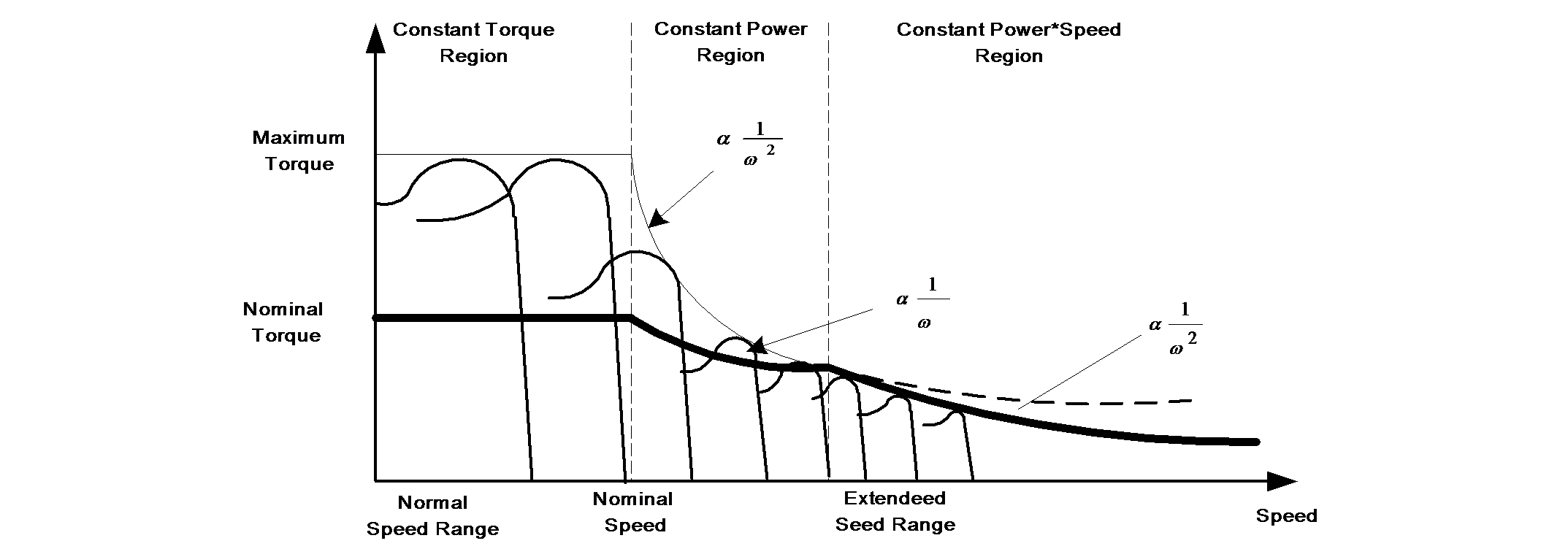
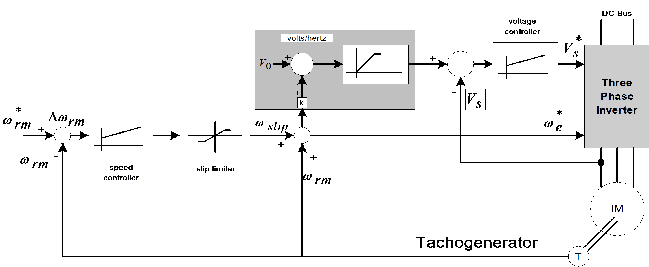
Figure 7.16. Maximal and Nominal Torque vs. Speed

Figure 7.17. Structure of a closed-loop scalar control with volts/hertz and slip regulation

Figure 7-17. shows a closed-loop speed control scheme, which uses volts/hertz and slip regulation.

The controlled slip strategy is widely used because the induction machine’s input power factor and torque to stator current ratio can both be kept high, resulting in better utilization of the available inverter current. When air-gap flux and slip speed are both held constant, the torque developed will be the same, but the efficiency is not as good as that obtained with air-gap flux and slip held constant. When the slip is held constant, the slip speed will vary linearly with the excitation frequency and the slope of the torque-speed curve on the synchronous speed side will decrease with the excitation frequency. These control methods have been well studied in the literature and it is not the subject of this thesis to give a more analytical insight into this field. Rather, we will turn now to the presentation of the more important vector control principle and the associated questions in AC motor control based on this principle.

7.8.2. Vector Control

Vector control is referring not only to the magnitude but also to the phase of these variables. Matrices and vectors are used to represent control quantities. This method takes into consideration not only successive steady states but also real mathematical equations that describe the motor itself. The control results obtained have a better dynamic for torque variations in a wider speed range. The space phasor theory is a method to handle the equations. Though the induction motor has a very simple structure, its mathematical model is complex, due to the coupling factors to be applied to a large number of variables, and to the non-linearities. Field Oriented Control (FOC) offers a solution to circumvent the need to solve high order equations and to achieve an efficient control with high dynamic. This approach requires more calculations than a standard U/f control scheme. This can be solved by the use of a calculation unit included in a Digital Signal Processor (DSP), and has the following advantages:

full motor torque capability at low speed,
better dynamic behavior,
higher efficiency for each operation point in a wide speed range,
decoupled control of torque and flux,
short term overload capability, four-quadrant operation.

7.8.2.1. The FOC Algorithm Structure

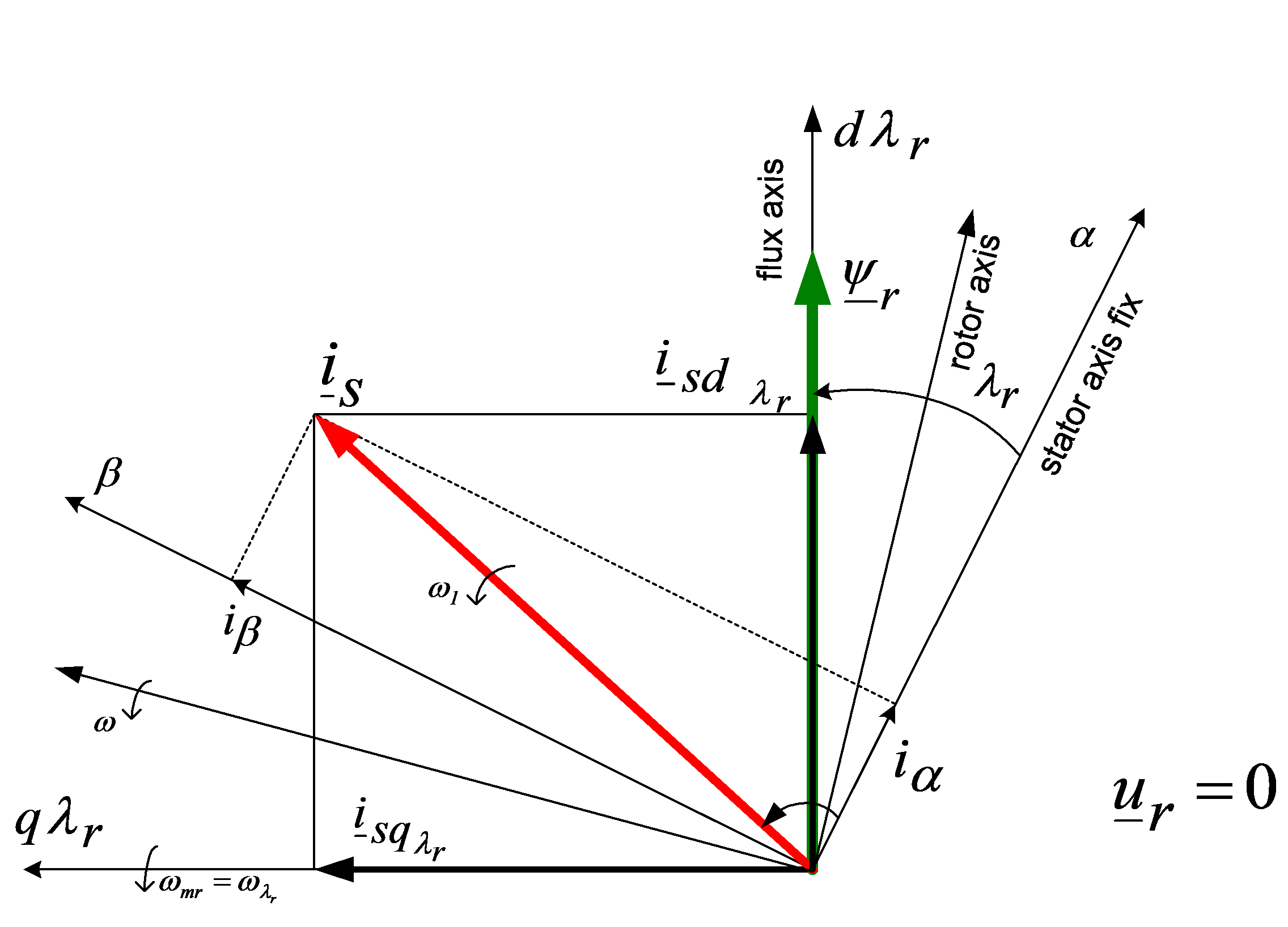
Figure 7.18. The vector diagram of FOC principle

FOC consists of controlling the components of the motor stator currents, represented by a vector, in a rotating reference frame d,q aligned with the rotor flux. The vector control system requires the dynamic model equations of the induction motor and returns the instantaneous currents and voltages in order to calculate and control the variables. Stator current and flux space vectors in the d,q rotating reference frame and the relationship of that with the , stationary reference frame can be seen in Figure 7-18. The control of induction machines must take place in an orthogonal reference frame that rotates with rotor flux angular velocity ( $ω_{λ_{r}}$ ) in such a way that the d $λ_{r}$ axes coincide with the instantaneous position of the rotor flux ${\bar{ψ}}_{r}$ . In this case the torque expression has just one term, a current multiplied by one flux. The orthogonal components of the fluxes will be zero. The current in the torque expression will not be other than the projection of stator current vector to the q $λ_{r}$ axes, and can be characterized as the active current. The stator current projection to the d $λ$ axes gives the magnetizing current of the motor. In this way the induction motor can be controlled by two separate loops: one for the reactive current (flux) and one for the active current (torque or speed), like a separately excited DC motor. The flux identification procedure defines the type of the control system.

There are very simple cases where the orientation flux and its position are determined by measurement. When this is not possible, in the majority of cases, the orientation quantities are determined by using the mathematical model of the induction machine expressed in the orthogonal co-ordinate system. A complex control system can define the orientation quantities in one co-ordinate system and control the motor to another. In Figure 7-19. the space phasor diagram of the induction machine with short circuited rotor windings is proposed. The most often used method is the one with rotor-resultant-flux orientation, because of the simple structure of the control loops and easy command variable calculation. The space phasor of the stator current is split into two components, which become control variables. Vector rotation techniques are used to transform three phase axes into rotating two-phase "d-q" axes. This two-phase rotation technique greatly simplifies the analysis, making it equivalent to analyzing separately excited DC motors, because in this case there are two independently controllable currents: the field current and the armature current. In a two-phase system $i_{α}$ and $i_{β}$ represent the stator current in the stationary reference frame where the axes of the two-phase system exactly match the “a” axis. To control field and torque independently, we must use the moving "d-q" co-ordinate system, rotated at the synchronous speed with respect to the stationary reference frame. Projecting $i_{- s}$ onto "d-q" yields the components $i_{s d λ_{r}}$ and $i_{s q λ_{r}}$ . To control these quantities the stator current vector must be oriented to "d-q", where $λ_{r}$ is the orientation angle. Let us omit the presentation of co-ordinate transformations related to the vector control strategy because they have been well described in the literature. We only summarize here the transformations that must be effectuated:

(a,b,c)(,) is the Clarke transformation, which outputs a two-co-ordinate time-variant system, and

(,)(d,q) is the Park transformation, which outputs a two co-ordinate time-invariant system.

This is the most important transformation in FOC. In fact, this projection modifies a two phase orthogonal system in a (d,q) rotating reference system.

Figure 7.19. Basic scheme of FOC for AC-motor

The (d,q) (,) projection is the inverse Park transformation.

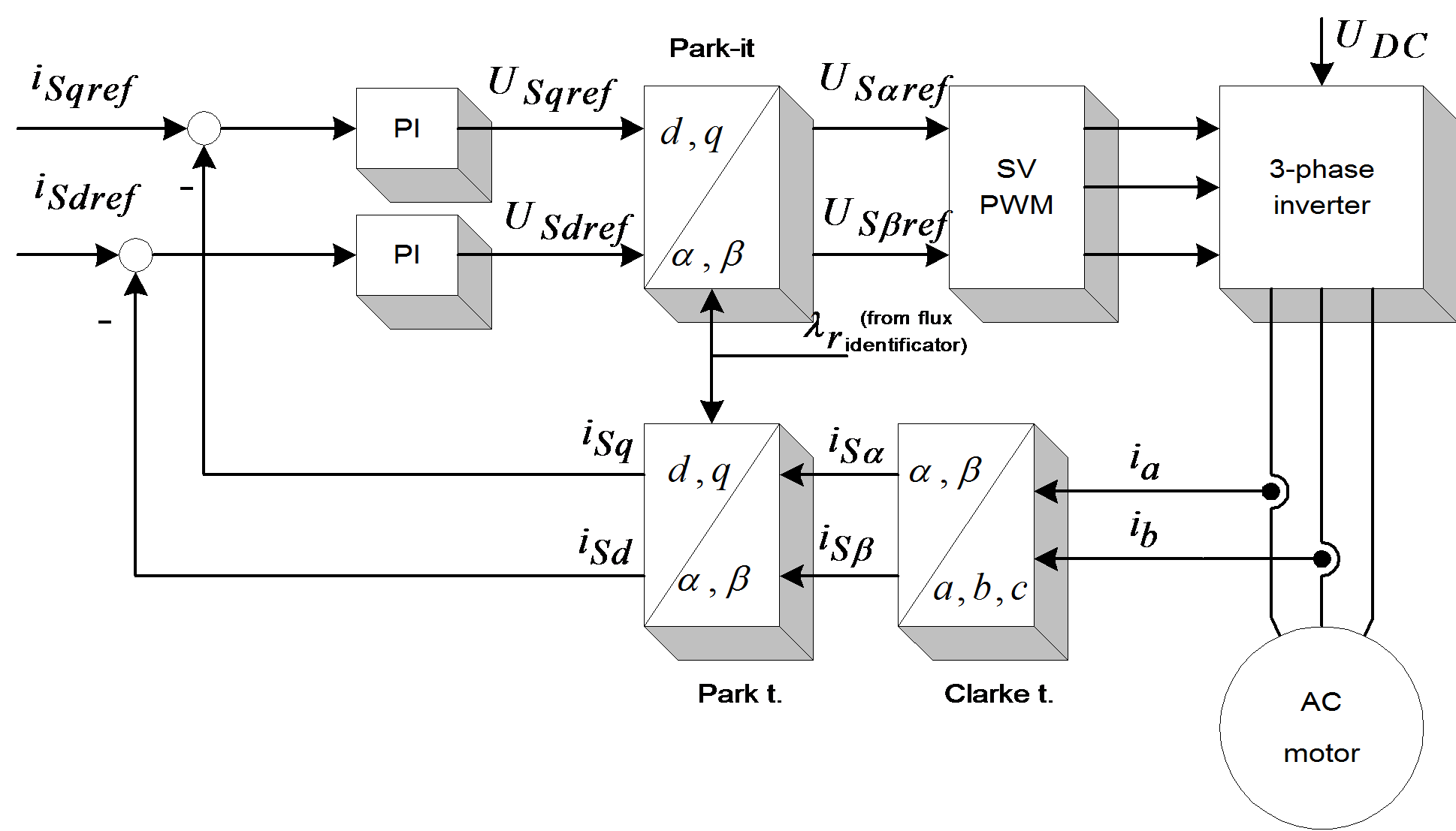
The outputs of this block are the components of the reference vector, which is the voltage space vector to be applied to the motor phases. Figure 7-20. summarizes the basic scheme of torque control with FOC. Two motor phase currents are measured, which feed the Clarke transformation module. The outputs of this projection are designated is and is. These two components of the stator current are the inputs of the Park transformation that gives the current in the d,q rotating reference frame. The isd and isq components are compared to the references (isd)ref (flux reference) and (isq)ref (torque reference). At this point, this control structure shows an interesting advantage: it can be used to control either synchronous or induction machines by simply changing the flux reference and obtaining the rotor flux position. As in the case of synchronous permanent magnet motors, the rotor flux is fixed (determined by the magnets) there is no need to create one. Hence, when controlling a PMSM, (isd)ref should be set at zero. As induction motors need rotor flux creation in order to operate, the flux reference must not be zero. This conventionally solves one of the major drawbacks of the “classic” control structures: the transferability from asynchronous to synchronous drives. The torque command (isq)ref could be the output of the speed regulator when we use a speed FOC. The outputs of the current regulators (usd)ref and (usq)ref are applied to the inverse Park transformation block. The outputs of this projection are (us)ref and (us)ref, which are the components of the stator vector voltage in the (,) stationary orthogonal reference frame. These are the inputs of the Space Vector PWM. The outputs of this block are the signals that drive the inverter. It is worth to remark that both the Park and the inverse Park transformation need the rotor flux position. Obtaining this rotor flux position depends on the AC machine’s type (synchronous or asynchronous). Some considerations with regards to rotor flux position for motors of the asynchronous type are the following. If the controlling method is based on the field-orientation principle, the identification of the oriented quantities is of crucial importance. This includes the calculation or prediction of the position and magnitude of the chosen flux, the control of the active and reactive currents in the d-q reference frame, and the recovery of these quantities in a,b,c quantities, which can control the motor through a static type frequency converter. The structure of the control system and the type of the frequency converter must be taken into consideration when making the important decision on which flux is to be used in orientation. The control systems differ not only in this respect, that is, which flux is used in orientation, but also in the identification procedure. There are very simple cases, when the orientation flux and its position are determined by measuring (direct vector control). When this is not possible, as in the majority of cases, the orientation quantities are determined by using the mathematical model of the induction machine (indirect vector control), written in the orthogonal co-ordinate system. This latter co-ordinate system can be oriented after another phasor (not only the flux phasor), in the scope of operation, with a simpler mathematical model.

Figure 7.20. Blockdiagram of a three Phases Asynchronous Motor Driver Using a FOC

Consequently, if a complex control system can define the orientation quantities in one co-ordinate system, and control the motor to another, the field-orientation cannot be used by itself. For this reason, the vector control terminology is appropriate for this system, rather than that of field-orientation. Another classification methodology can also be adapted to a field-oriented control system, based on the determination of the field-orientation quantities, when the parameters are identified on-line. This method means real-time identification and tracing of process quantities like the resistance of the rotor and the changes of the rotor’s time constant. This method is applicable to such systems where the torque has a low changing rate. A more efficient method is where parameter identification is determined off-line, with the help of a mathematical model of the motor, the method of previously testing the machine, is applicable on a large operation scale.

The electric torque of an AC induction motor can be described by the interaction between the rotor currents and the flux wave resulting from the stator current induction. Since the rotor currents cannot be measured with cage motors, this current is replaced by an equivalent quantity described in a rotating co-ordinate system called d,q following the rotor flux. The instantaneous flux angle $λ_{r}$ is calculated by the motor flux model, which will be given later. isd and isq, the stator current components in the d,q frame, are obtained directly from ia, ib and ic, the fixed co-ordinate stator phase currents, with the Park transformation:

$[\begin{matrix} i_{s d} \\ i_{s q} \end{matrix}] = [\begin{matrix} \cos λ_{r} & \cos (λ_{r} - 2 π / 3) & \cos (λ_{r} + 2 π / 3) \\ - \sin λ_{r} & - \sin (λ_{r} - 2 π / 3) & - \sin (λ_{r} + 2 π / 3) \end{matrix}] [\begin{matrix} i_{s a} \\ i_{s b} \\ i_{s c} \end{matrix}]$

(7.118)

In steady-state conditions the stator current is defined in the above mentioned rotating system is considered constant, as well as the magnetizing current imr representing the rotor flux, isq being equivalent to the motor torque. isd is linked to imr [16] and [18] with the following equation:

$i_{s d} = i_{m r} + T_{r} \frac{d i_{m r}}{d t}$

(7.119)

where $T_{r}$ is the rotor time constant. This system together with the angle transformations, changes the induction motor into a machine very similar to a DC motor where imr corresponds to the DC motor’s main flux, and isq to the armature current. The field-oriented control method achieves the best dynamic behavior, whereby the lead and disturbance behavior can be improved with shorter control cycle times. The field oriented control method is a de facto standard to control an induction motor in adjustable speed drive applications with quickly changing load as well as reference speeds. Its advantage is that by transforming measurable stator variables into a system based on field co-ordinates the complexity of the system can be enormously reduced. As a result, a relatively simple control method, very similar to that of a separately exited DC motor, can be applied. The role of the DSP in such a system is to translate the stator variables (currents and angles) into a flux model as well as to compare the values with the reference values and update the PI controllers. After back transformation from field to stator co-ordinates, the output voltage will be impressed to the machine with a symmetric or asymmetric PWM, whereby the pulse pattern is computed on-line by the DSP or a hardware generated space vector method. In some systems the position is measured by an encoder. This extra cost can be avoided by implementing an observer model, or, in particular cases, a Kalman filter. These algorithms are complex and, therefore, require a fast processor. A fixed-point DSP is able to perform the above controls with short cycle times. Let us repeat here the basic equations of field orientation, which are deduced in [18]. Substituting the rotor current in the rotor voltage equation and considering the magnetizing current equal to the rotor flux divided by main the inductance, we can express the d-q components of the stator current phasor as follows:

${\begin{cases} (_{i_{s d}) λ_{r}} = i_{m r} + T_{r} \frac{d i_{m r}}{d t} \\ (_{i_{s q}) λ_{r}} = T_{r} ((_{ω) λ_{r}} - ω) i_{m r} \end{cases}$

(7.120)

The d component of the stator current vector is influenced by the rotor-flux amplitude variation, and the q component by the relative speed between the rotor-flux space-phasor and the rotor’s spatial position. Looking at the equation (7.120), we can notice that whenever the rotor-flux magnitude is not constant, the d component of the stator current contains a new element, proportional to this flux variation, and respectively, to the magnetizing current (delay element). The electromagnetic air-gap torque can be calculated from the flux-oriented variables as follows:

$m_{e} = \frac{3}{2} p \frac{1}{1 + σ_{r}} ℑ m ({\bar{i}}_{s} {\bar{ψ}}_{r}^{*})$

(7.121)

If the variables are all rotor-flux-oriented, the following expressions can be obtained:

$m_{e} = K_{M r} ψ_{r} {(i_{s q})}_{λ r}, w h e r e K_{M r} = \frac{3}{2} \frac{p}{1 + σ_{r}} = \frac{K_{M}}{1 + σ}$

(7.122)

Figure 7.21. Flux identification model in the case of a rotor-flux–oriented coordinate system

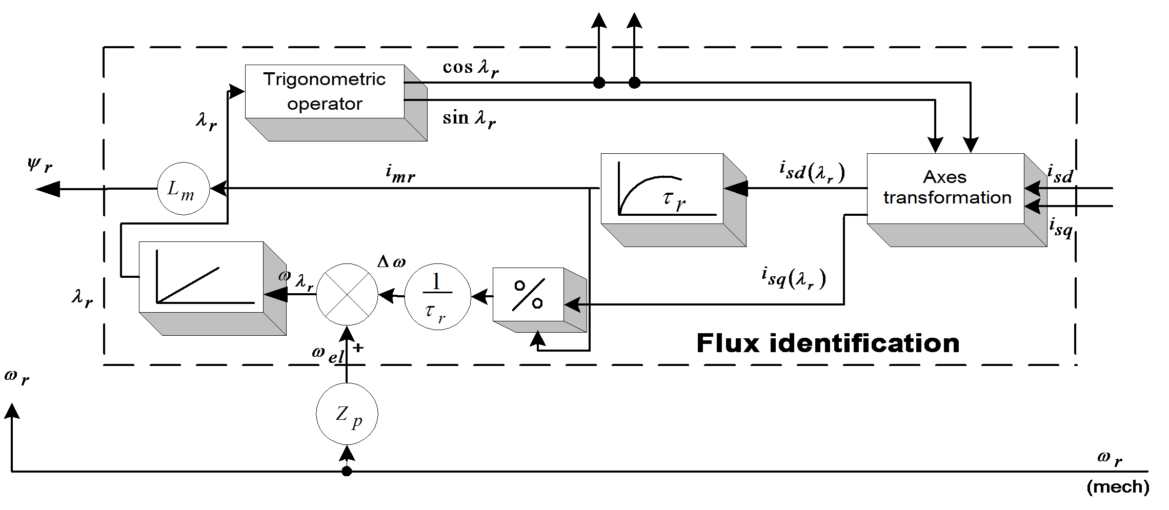
The rotor-flux-oriented components of the stator current space phasor $i_{s d λ_{r}}, i_{s q λ_{r}}$ can serve for the control of rotor flux and the machine torque, respectively. Let us take a look now at the calculation of the orientation quantities based on the above-deducted equations. As the input stator components must be oriented and the orientation variables appear only at the output of this block, internal calculations to determine the trigonometric functions are needed. The structural scheme of the flux identification is given in Figure 7-21. The stator current components are field-oriented. The two non-linear differential equations prove to be stable under all operating conditions and their continuous on-line solution on a DSP does not raise problems. It is more advantageous to use stator currents instead of voltages, due to their reduced harmonic content. This is the reason why at stator frequencies lower than 100 Hz, a sampling time of 1ms and a 10-bit resolution A/D converter are permitted. The stator resistance and leakage inductance have no influence on the orientation-field calculation, as the feedback loop is independent of the stator voltage model. Of real interest are the rotor parameters, especially the time constant $T_{r}$ , influenced by the rotor resistance (varying with the temperature), and the iron-core saturation. The torque calculation is also dependent on Lm and on the rotor leakage coefficient $σ_{r}$ . In order to achieve higher speeds, higher than the nominal values, the stator frequency has to be increased. In high frequencies the stator resistance can be neglected. If the flux magnitude variation is also neglected, the voltage equation becomes very simple: ${\bar{u}}_{s} \approx j ω_{1} {\bar{ψ}}_{s}$ , where $ω_{1}$ is the synchronous frequency. It is obvious that if the flux is kept constant, the limit voltage of the converter is reached at a certain stator frequency. Thus the flux must be reduced if further speed increase is needed. Under such operating conditions, in the so-called field weakening region, the stator voltage is kept approximately constant at its maximum.

7.9. Summary

When the rotor is short circuited and if the rotor flux magnitude is constant then the rotor current vector is perpendicular to the flux phasor direction. In the equation (7.123) there is summarized the two cases of rotor flux identification are summarized. First, when the rotor flux magnitude is kept at a constant value, and, in the second case, it can change. In the latter case a time lag appears in the equation of the flux generation component of the stator current vector.

$\begin{matrix} f l u x c o n s t : & \begin{array}{l} {(i_{s d})}_{λ_{r}} = i_{m r} \\ {(i_{s q})}_{λ_{r}} = T_{r} ({(ω)}_{λ_{r}} - ω) i_{m r} \end{array} & f l u x v a r i a b l e : & \begin{array}{l} {(i_{s d})}_{λ_{r}} = i_{m r} + T_{r} \frac{d i_{m r}}{d t} \\ {(i_{s q})}_{λ_{r}} = T_{r} ({(ω)}_{λ_{r}} - ω) i_{m r} \end{array} \end{matrix}$

(7.123)

where

$i_{m r} = \frac{i_{s}}{\sqrt{1 + T_{r}^{2} {({(ω)}_{λ_{r}} - ω)}^{2}}} = \frac{i_{s}}{\sqrt{1 + T_{r}^{2} {(Δ ω)}^{2}}}$

(.7.124)

The reactive current is influenced by the rotor flux amplitude variation, and the active one by the relative speed between the rotor-flux space phasor and the rotor’s spatial position. Comparing the above two equations, it can be noticed that whenever the rotor-flux amplitude is not constant, the reactive component of the stator current contains a new element, proportional to this flux variation and to the magnetizing current variation, respectively.

7.9.1. The Matlab/Simulink Model of the Field Oriented Control

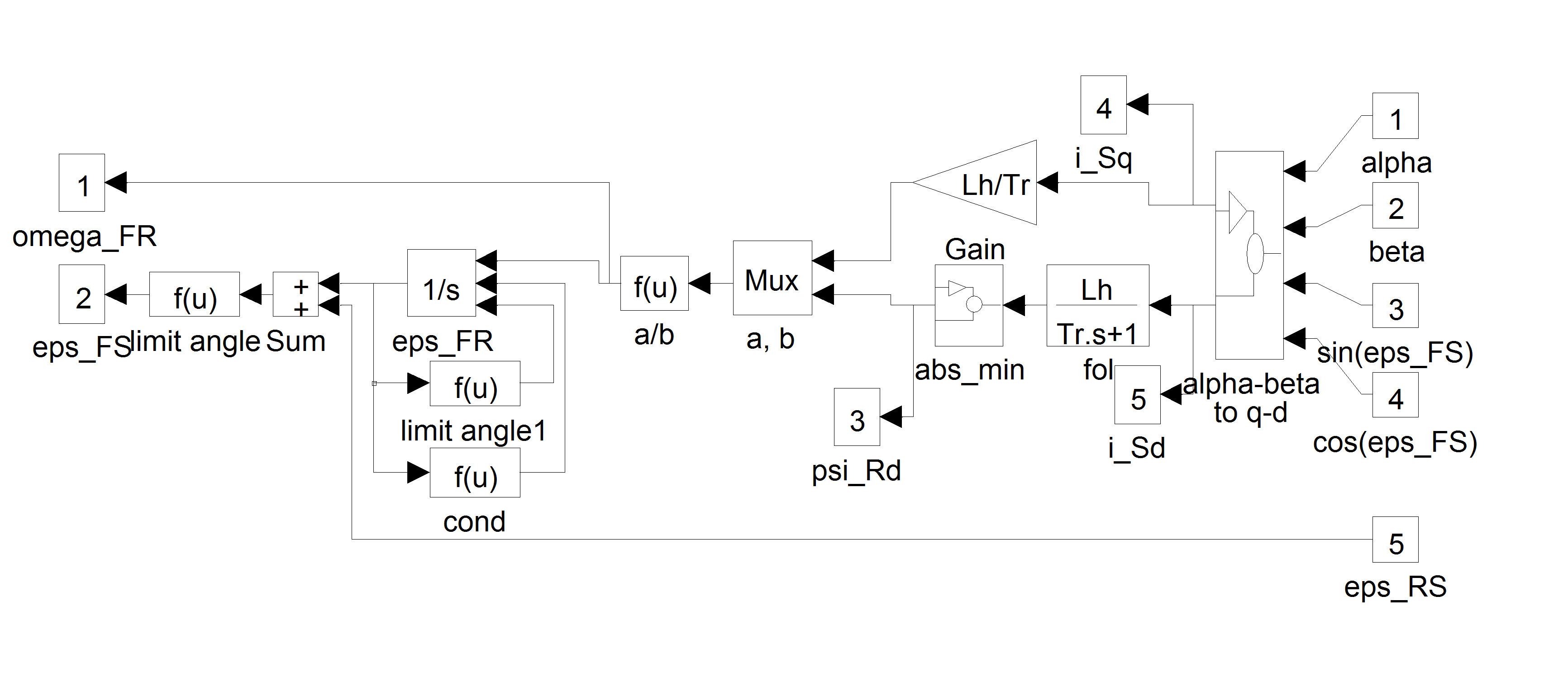
Figure 7.22. SIMULINK model of the rotor flux identification

Let us give an overview from the point of view of simulation, on how the FOC can be implemented in Matlab/Simulink graphical development system. The differential equations treated in [16], [14], and [18] were taken into account. The usage of symbols was taken from the dSpace realization, to avoid possible misunderstanding. For the complete controller, the controlling parameters described in [15] were adapted. A slight modification to the structure of the theoretical flux model was effectuated. The flux model can be seen in Figure 7-22. Before carrying out the division by “psiRd” ( $ψ_{r d}$ ), we have to make sure that its value is not zero, otherwise an infinite value gets into the system, which, in turn, causes all further calculations to "blow up". To make sure that this does not happen, we must "part" $ψ_{r d}$ from zero by a small value. This task is done by the block "abs min". This block sets psi_offset as a minimal absolute value for $ψ_{r d}$ . This means, that either $ψ_{r d}$ <psi_offset or $ψ_{r d}$ >psi_offset must be true. The value of psi_offset should be set to a small value, so that psi_offset<<psi_Rd_ref, where psi_Rd_ref is the reference, which is in our case a constant value. This is in fact a modification, which is implicitly included in the software, since in the software a division by 0 is saturated to the maximal or the minimal value of the fractional. The sine and cosine values of the transformation angle eps_Rd ( $ε_{r d}$ ) are given twice: once for transformation, and once for inverse transformation. Avoiding this by calculating sine and cosine values only once, and using these values directly for both directions of calculation, gave results to a much faster working flux model. Let us show now the whole control system in Figure 7-24., and the FOC part of it in Figure 7-28.