Chapter 8. Models of Friction
8.1. Early Models of Friction
When one would like to examine the current achievements and theories, it worth to look back to the past and evaluate, how our predecessors interpreted the same problem. Below, a short summary is given concentrated only on the development of friction models, from the middle ages till the mid 20th century.
8.1.1. The first friction model
It is interesting, but probably not that surprising, that the first friction model came from Leonardo Da Vinci (1452-1519). Leonardo measured the force of friction between objects on both horizontal and inclined surfaces and he soon recognized the difference between rolling and sliding friction and the beneficial effect of lubricants.
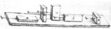
As Figure 8-1 shows, Leonardo was curious of the influence of the apparent area. He wrote to his notebooks: “The friction made by the same weight will be of equal resistance at the beginning of its movement although the contact may be of different breadths and lengths.” The above observations are entirely in accord with the first two laws of friction. (see chapter 1.4.9)
Leonardo introduced first the coefficient of friction as the ratio of the force of friction and the normal load, however he assumed, that for smooth surfaces “every frictional body has a resistance of friction equal to one quarter of its weight.”
8.1.2. A more scientific approach
Robert Hook (1635-1703), inspired by the famous Stevin’s chariot [141] – a ship-like vehicle on wheels with masts, sails and other convenient riggings – discussed rolling friction and recognized two components: “…The first and chiefest, is the yielding, or opening of the floor, by the weight of the wheel so rolling and pressing; and the second, is the sticking and adhering of the parts of it to the wheel;…”
He further distinguished between the role of recoverable and non-recoverable deformation, and also discussed the question of sticking and adhesion.
Much of the scientific work of friction was initiated by Guillaume Amontons (1663-1705) of France. His experiments and interpretation of results were published in a classical paper presented to the Académie Royale in 1699.
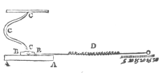
The apparatus used by Amontons in his experiment is shown in Figure 8-2. The test specimens of AA and BB were loaded together by various springs denoted by CCC, while the force require to overcome friction and initiate sliding was measured on the spring balance D.
8.2. Friction phenomena
Friction is the tangential reaction force between two surfaces in contact. Physically these reaction forces are the results of many different mechanisms, which depend on contact geometry and topology, properties of the surface materials of the bodies, displacement and relative velocity of the bodies and presence of lubrication.
Contact surfaces are very irregular at microscopic level (see in Figure 8-3).
It can be visualized as two rigid bodies that make contact through elastic bristles (see in Figure 8-4).
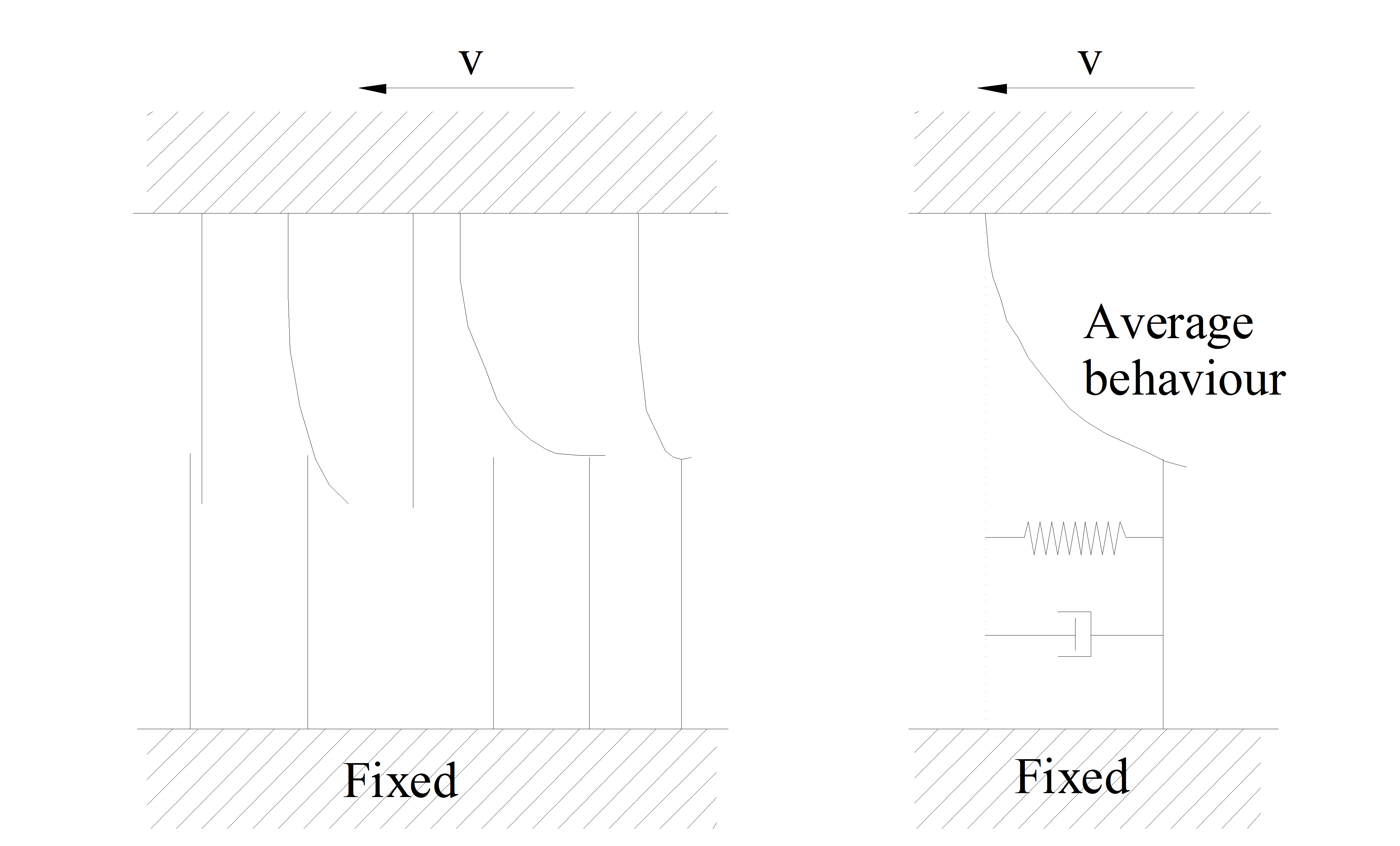
When tangential force is applied, the bristles will deflect like springs and dampers, giving raise to microscopic displacement (stick). If the displacement becomes too large, the bristles break (see in Figure 8-5).
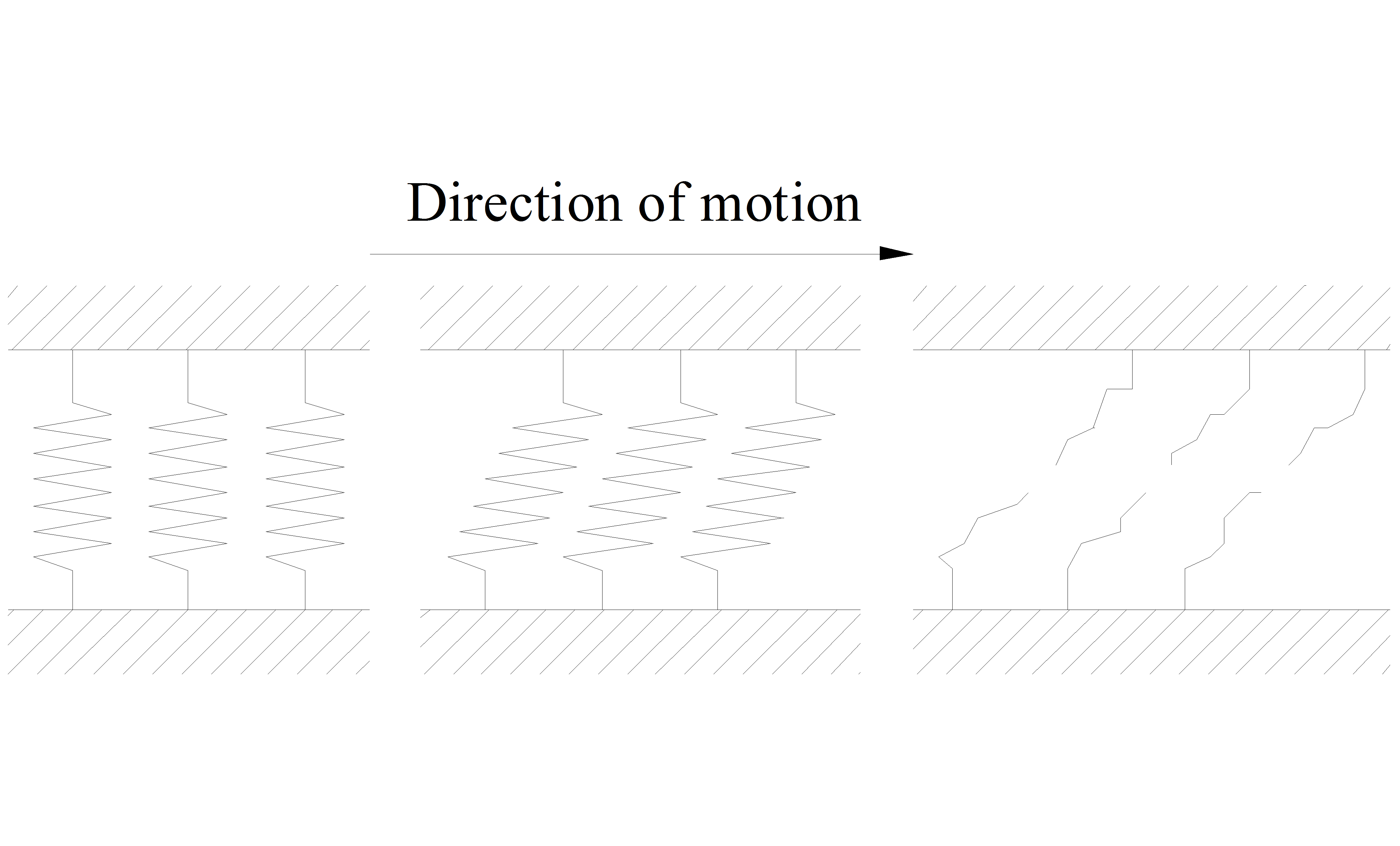
At this break-away displacement macroscopic sliding (slip) starts. The friction force where this occurs is called break-away force. The average deflection of the bristles corresponds to the internal state of the dynamic friction models. [10].
In dry sliding contacts between flat surfaces friction can be modeled as elastic and plastic deformation forces of microscopical asperities in contact. The asperities each carry a part fi of the normal load FN. If we assume plastic deformation of the asperities until the contact area of each junction has grown large enough to carry its part of the normal load, the contact area of each asperity junction is:
|
|
(8.1) |
where H is the hardness of the weakest material of the bodies in contact. The total contact area thus can be written
|
|
(8.2) |
This relation holds even with elastic junction area growth, provided that H is adjusted properly. For each asperity contact the tangential deformation is elastic until the applied shear pressure exceeds the shear strength τy of the surface materials, when it becomes plastic. In sliding the friction force thus is:
|
(8.3) |
and the friction coefficient:
|
(8.4) |
The friction coefficient is independent on the normal load or the velocity in this case. Consequently it is possible to manipulate friction characteristics by deploying surface films of suitable materials on the bodies in contact. [5].
As with many problems in the physical sciences, friction can be approached by using forces or by using energy. The best known model for friction that utilizes the force approach has been postulated by Bowden and Tabor. They suggested that surfaces adhere to form junctions and the friction force is directly related to the force needed to shear these junctions. The normal load FNis supported by the total contact area A of the deformed surfaces. If τjct is the shear strength of the adhesive junctions, then the frictional force:
|
(8.5) |
where PY is the yield pressure. Thus the coefficient of friction:
|
(8.6) |
Estimates of the friction coefficients from this expression have been reported as μ=0.2-0.3.
This model is based on the assumption of homogeneous and isotropic materials and uses a limited number of variables. Basic material characteristics tend to be neglected in most available model of friction. Microstructural information which significantly influences material behaviour is generally omitted.
Some plastic deformations always occur near the surfaces of sliding materials. Therefore plastic deformation and associated parameters such as microstructure as mentioned before are important parameters in setting up a more realistic friction model. P. Heilman and D. A. Rigney have presented an energy based model of friction. It is assumed that the frictional work is approximately equal to the plastic work done, or:
|
(8.7) |
where τ(γ) is the shear stress, γ is the shear strain and V is the deformed volume near to the surface. This approach is applicable for metals and for some polymers and ceramics, which can deform plastically under compressive loading.
In dry rolling contact, friction is the result of a non-symmetric pressure distribution in the contact. The pressure distribution is caused by elastic hysteresis in either of the bodies, or local sliding in the contact. For rolling friction the friction coefficient is proportional to the normal load as
|
(8.8) |
The elastoplastic characteristics of dry friction can be described by hysteresis theory.
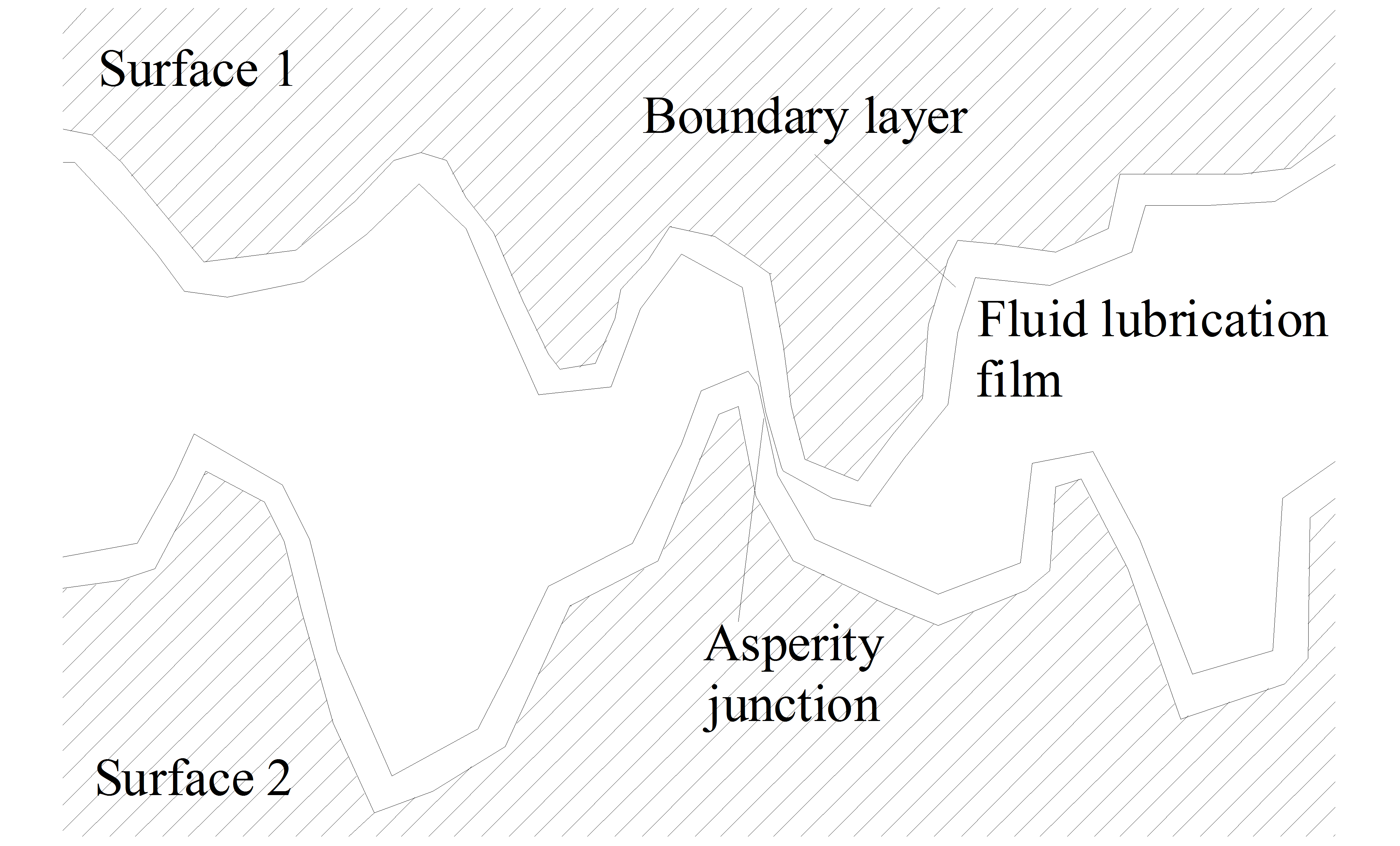
Other physical mechanisms appear when lubrication is added to the contact. For low velocities, the lubricant acts as a surface film, where the shear strength determines the friction. At higher velocities at low pressures a fluid layer of lubricant is built up in the surface due to hydrodynamic effects. Friction is then determined by shear forces in the fluid layer. These shear forces depend on the viscous character of the lubricant, as well as the shear velocity distribution in the fluid film. Approximate expressions for the friction coefficient exist for a number of contact geometries and fluids. At high velocities and pressures the lubricant layer is built up by elastohydrodynamic effects. In these contacts the lubricant is transformed into an amorphous solid phase due to the high pressure. The shear forces of this solid phase turn out to be practically independent of the shear velocity. The shear strength of a solid lubricant film at low velocities is generally higher than the shear forces of the corresponding fluid film built up at higher velocities. As a result the friction coefficient in lubricated systems normally decreases when the velocity increases from zero. When the thickness of the film is large enough to completely separate the bodies in contact, the friction coefficient may increase with velocity as hydrodynamic effects become significant. This is called the Stribeck effect.
Film thickness is a vital parameter in lubricated friction. The mechanisms underlying the construction of the fluid film includes dynamics, thus suggesting a dynamic friction model. Contamination is another factor that adds complication. The presence of small particles of different materials between the surfaces give rise to additional forces that strongly depend on the size and material properties of the contaminants.
This short expose of some friction mechanisms illustrate the difficulty in modeling friction. There are many different mechanisms. To construct a general friction model from physical first principles is simply not possible. Approximate models exist for certain configurations. What we look for instead is a general friction model for control applications, including friction phenomena observed in those systems.
8.2.1. Friction - General observations
Talking about friction in general, we can summarize the basic, well-known properties in five points according to [111].
1.) In any situation where the resultant of the tangential forces is smaller than some force parameter specific to that particular situation, the friction force will be equal and opposite to the resultant of the applied forces and no tangential motion will occur.
2.) When tangential motion occurs, the friction force always acts in a direction opposite to that of the relative velocity of the surfaces.
3.) The friction force Ff is proportional to the normal force F. This relationship enables us to define the coefficient of friction :
|
F = F |
(8.9) |
Alternatively this law can be expressed in terms of a constant angle of repose or frictional angle , defined by:
|
tan = |
(8.10) |
It may readily be shown that is the angle of an inclined plane such, that any object, whatever its weight placed on the plane will remain stationary, but that if the angle is increased by any amount whatever, the object will slide down.
4.) The friction is independent the apparent area of contact Aa. Thus, large and small objects have the same coefficients of friction.
5.) The friction force is independent of the sliding velocity v. This implies that force required to initiate sliding will be the same as the force to maintain sliding at any specified velocity.
These frictional properties are widely used in the everyday life and often in the engineering practice. Despite, unfortunately, we can say they are simply and solely good approximations. The research of friction is going on, and tribology still contains many uncovered areas. What we can be already sure about is that the real picture is far more complex and many times surprisingly different from the given points above.
8.2.2. Origin of friction
The model described above dates back to the 18th century and still with us since the scientific achievements of Amontons and Coulomb. Thanks to the technological evolution the 20th century brought to life many new tools and methods backing up tribological researches and made possible to reconsider the interpretation of friction.
The Coulomb type model suffers from two great mistakes. On one hand the whole model lays basically on the roughness theory and claims that friction is based almost solely on surface roughness. The reason for this is simple. By that time special equipment and supplementary knowledge were missing to find out the connection between friction and adhesion. On the other hand in this way this model also fails to demonstrate convincing the dissipative nature of friction.
Although there were theories pointing towards the right direction [140], we can say that the real breakthrough happened during World War II, in 1943, in Australia. It was the series of experiments carried out Bowden and Tabor [24], which provided experimental evidence for earlier adhesion theories, and which gave a chance at last to explain frictional losses.
They studied the behavior of concentrated contacts – a sphere in contact with a flat [23], [24], [25]. As the surfaces were “smooth” they modeled the noncomformal contact of a single asperity so that the geometric area became a fair approximation of the real area. They used metal indium what is not only known as a very soft material (its hardness is about one quarter of the hardness of lead) but is also relatively inert, thus, the effect of oxide films is negligible.
They made three important observations.
First, the area of geometric contact was proportional to the load. The deformation was clearly plastic. This at once indicated that for extended surfaces each asperity deformed plastically under the load that it born, thus, the total area of contact was proportional to the total load.
The second was that the indium actually stuck with the other surface and a small, finite normal force was required to pull it off. Clearly strong interfacial bonds were formed. This phenomenon referred to adhesion between the two contacting surfaces.
The third observation was that in sliding there was plastic flow as the indium sheared away in its adhered region. When the system was inverted, and a hard sphere slid over indium they observed an additional resistance to sliding due to the work of plastically grooving the indium surface.
They experienced similar results with other material pairs. Extending the results of these experiments they attributed the friction to two factors [24], [25]. Which later works of Rabinowicz added two more to [111].
Friction is due to four main factors:
-
The adhesion of one surface to the other.
-
Plowing of the softer surface by asperities on the harder.
-
Roughness of the surfaces.
-
Electrical components.
In the previous chapters we took a look at to the origin and cause of friction as well as its forms of appearance. Below, we try to summarize the different approaches used for modeling this phenomenon.
8.3. Simple elements
Static models are mostly simple mathematical representations of certain frictional behaviors. They do not deal with friction as a complex process, only with some of its sub processes, such as frictional force at rest i.e. static friction, friction as a function of steady-state velocity, etc.
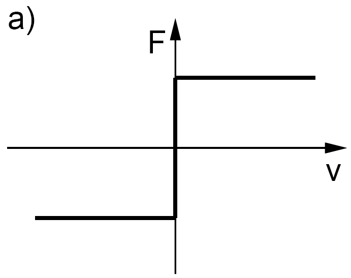
8.3.1. Coulomb friction
The easiest and probably the most well known model is the so-called Coulomb friction model. Though it greatly over simplifies the frictional phenomena it is widely used in the engineering world, when dynamic effects are not concerned. Also, the Coulomb model is a common piece of all more developed models. The Coulomb friction force Fc is a force of constant magnitude, acting in the direction opposite to motion:
When:
|
(8.11) |
|
|
(8.12) |
Where FN is the force pressing surfaces together and μ is the frictional factor. μ is determined by measurements under certain conditions. One of the biggest problems of the Coulomb model is, that it cannot handle the environment of zero velocity, hence the properties of motion at starting or zero velocity crossing, i.e. static and rising static friction. To apply the model for those cases a μ0 factor has been introduced. In case of starting the motion it replaces μ in Equation (8.12) until the process arrives to steady state. The values of μ and μ0 can be found in any major physics or engineering tabulations for different material pairs in both dry and lubricated conditions. The first tabulations of those kinds date back to the beginning of 18th century. Note, that though this is the simplest and fastest way to calculate the frictional force, this method can suffer from the error up to 20%.
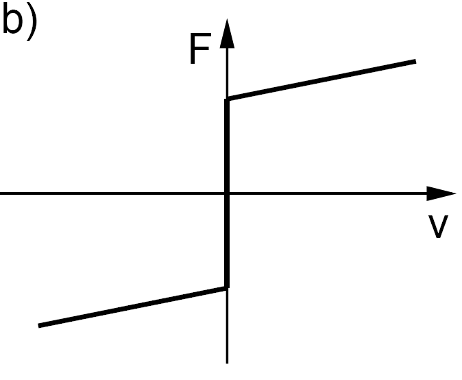
8.3.2. Viscous friction
The viscous friction element models the friction force as a force proportional to the sliding velocity:
When:
|
(8.13) |
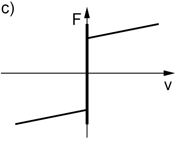
8.3.3. Static friction
Static friction is a force of constraint:
When
|
(8.14) |
where Fs is the static friction force, an additional upload on Fc, the Coulomb friction force.
8.3.4. Stribeck effect
The Stribeck curve is a more advanced model of friction as a function of velocity. Although it is still valid only in steady state, it includes the model of Coulomb and viscous friction as built-in elements.
8.3.5. Presliding displacement
The presliding displacement was studied and modeled first by Dahl [40]. Recalling xxx he gives:
|
(8.15) |
where Ff(x) is the friction force as the function of presliding displacement, kt is the stiffness of the material and x is the displacement. kt is a material property, but can be calculated using Equation (8.15) such a way, that x is in the range of 1-50 [μm].
8.3.6. Rising static friction and dwell time
There are several models available describing this phenomenon. The empirical model of Kato [85] is:
|
(8.16) |
where is the ultimate static friction, i.e. the magnitude of static friction after a long time of rest, FC is the Coulomb friction at the moment of arrival to stuck, and m are empirical parameters in the range of 0.04 to 0.64 and 0.36 to 0.67 respectively. Small means long rise time and thus resists thick slip. Examining non-conformal contacts Amstrong-Hélouvry finds = 1.66 and m = 0.65 [6].
Another model presented by Amstrong-Hélouvry [6] eliminates the use of FC as the starting point of the static friction rise. Thus the model has one fewer parameter than that of Equation (8.16).
|
(8.17) |
where is the level of static friction at the beginning of the nth interval of slip, i.e. breakaway, is the level of static friction at the end of previous interval of slip, is the ultimate static friction, is an empirical parameter. Note that will be different in physical dimension from that of Equation (8.16).
8.3.7. Frictional memory
Frictional memory is modeled simply as a time lag:
|
(8.18) |
where Ff(t) is the instantaneous friction force, Fvel() is friction as a function of steady state velocity and t is the lag parameter. Measuring frictional time lag, Hess and Soom [75] find them in the range of 3 to 9 ms depending on the load and lubrication. They also show that the lag increasing with increasing lubricant viscosity and increasing contact load. However, it appears to be independent from oscillation frequency.
8.4. Complex models
Complex models are mostly built upon the simple model elements with additional features, which can handle dynamic behavior. Yet the science of tribology is still far from having a complete picture on how friction works in all extent, therefore these models are mostly based on empirical experiences, rather than deep scientific background.
8.4.1. Steady state models
8.4.1.1. Stribeck curve
The model below was employed by Hess and Soom [75].
|
(8.19) |
where the Coulomb, viscous and static friction is denoted by FC, Fv and Fs respectively. vs is the characteristic velocity of the Stribeck curve. Hess and Soom reported systematic dependence of Fv and vs on lubricant and loading parameters.
Another proposal for modeling the Stribeck effect is a linearized exponential equation of Bo and Pavelescu [21]. The viscous friction term was added by Armstrong-Hélouvry [9].
|
(8.20) |
where δ is an additional empirical parameter. In the literature surveyed by Bo and Pavelescu [21] they find the range of δ from 0.5 to 1. Armstrong-Hélouvry [6], [8] employs δ = 2 and Fuller [57] suggest δ = very large for systems with effective boundary lubricants. Applying δ = 2 the exponential model, Equation (8.20) becomes Gaussian model, which is nearly equivalent of the Lorentzian model of Equation (8.15).
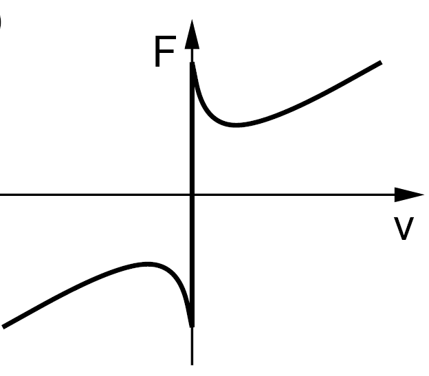
8.4.1.2. Tustin model
Another simple representation of the Stribeck curve is the Tustin model [144]. The model captures the basic frictional phenomenon and simply superposes them on one another. The three features are the Coulomb friction FC, the static friction Fs with the downward bend of the negative viscous effect determined by α and the viscous friction Fv.
|
(8.21) |
Linearizing the Tustin model we get:
|
(8.22) |
This model although a linear one, leads to a precision of approximated friction only up to 85% in the region where the velocity comparable to its square root. In other cases where the system velocity is not so very low, another model should be used.
8.4.2. Dynamic models
8.4.2.1. Seven-parameters friction model
A popular approach is simply sewing together the already existing model elements. This is how the seven-parameters model works. Each of the seven parameters of the model represents a different friction phenomenon as presented in Table 8.2. They value principally depends upon the mechanism and the lubrication conditions, but typical values may be offered based on the works of [6], [27], [57], [75], [85], [105].
The friction is given by:
Not sliding (presliding displacement)
|
(8.23) |
Sliding (Coulomb + viscous + Stribeck curve friction with frictional memory)
|
(8.24) |
Rising static friction (frictional level at breakaway):
|
(8.25) |
Where:
|
Ff() |
is the instantaneous friction force |
|
FC |
(*) is the Coulomb friction force |
|
Fv |
(*) is the viscous friction force |
|
Fs |
is the magnitude of the Stribeck friction (frictional force at breakaway is FC+Fs) |
|
Fsa |
is the magnitude of the Stribeck friction at the end of the previous sliding period |
|
Fs |
(*) is the magnitude of Stribeck friction after a long time at rest (with a slow application of force) |
|
kt |
(*) is the tangential stiffness of the static contact |
|
vs |
(*) is the characteristic velocity of Stribeck friction |
|
L |
(*) is the time constant of frictional memory |
|
(*) is the temporal parameter of the rising static friction |
|
|
t2 |
is the dwell time, time at zero velocity |
|
(*) |
marks friction model parameters, other variables are state variables |
|
Parameter range |
Parameter depends upon |
|
|
FC |
0.001 0.1FN |
Lubricant viscosity, contact geometry and loading |
|
Fv |
0 very large |
Lubricant viscosity, contact geometry and loading |
|
Fs |
0 0.1FN |
Boundary lubrication, FC |
|
kt |
1/x(FC+Fs) x1 50 [m] |
Material properties and surface finish |
|
vs |
0.00001 0.1 [m/s] |
Contact geometry and loading |
|
L |
1 50 [ms] |
Lubricant viscosity, contact geometry and loading |
|
0 200 [s] |
Boundary lubrication |
|
Friction model |
Predicted/observed behavior |
|
Viscous |
Stability at all velocities and at velocity reversals |
|
Coulomb |
No stick-slip for PD control No hunting for PID control |
|
Static + Coulomb + Viscous |
Predicts stick-slip for certain initial conditions under PD control Predicts hunting under PID control |
|
Stribeck |
Needed to correctly predict initial conditions leading to stick-slip |
|
Rising static friction |
Needed to correctly predict interaction of velocity and stick-slip amplitude |
|
Frictional memory |
Needed to correctly predict interaction of stiffness and stick-slip amplitude |
|
Presliding displacement |
Needed to correctly predict small displacements while sticking (including velocity reversals) |
Parameter identification. The parameters, which represent a non-linear relationship with the friction force, cannot be identified by using linear methods. Kim et al proposes a possible non-linear identification method for the seven parameter model, the Accelerated Evolutionary Programming (AEP) [88] and gives the description as outlined below. AEP is a stochastic optimization technique for finding the extrema of an arbitrary function. A simple optimization problem can be stated as: determine the values of the ordered set of n parameters
|
(8.26) |
which minimize/maximize the cost function f(z). AEP is a genetic algorithm type method, working with parent/child interactions to converge to the best solution. It uses two variation operators. One of them, the direction operator determines the direction of the search according to the fitness score. The other one is a zero-mean Gaussian operator, used a perturbation added to a parent in order to generate an offspring. AEP also uses a further “age” variable to enhance the diversity of the search and to prevent individuals to remain in the local minima. The Gaussian operator is incorporated with both the direction operator and the variable age. Unlike another genetic methods, AEP generates only one child from its parent. New parents then are selected in one-to-one competition between parent and its child. An offspring is selected if the child wins in the competition with its parent. AEP incorporates the direction of evolution and the age concept into the vector to be optimized in order to increase the convergence speed without loosing the diversity. Thus it brings Equation (8.26) into the form of
|
(8.27) |
where for allis the evolving direction of the jth parameter in the ith vector, and agei denotes the duration of the life in an integer type in the ith vector. The following two rules are applied for perturbing the parents to generate their offspring.
Rule 1
When ,
then ,
or else ,
|
(8.28) |
Rule 2
When ,
then ,
or else ,
,
|
(8.29) |
where denotes the jth parameter in the ith vector among Np vectors at the kth generation, denotes the evolving direction of , is a realization of a Gaussian-distributed random variable, which is polarized in the direction of , and i, i = 1, 2 are positive constants. Rule 1 indicates that if the performance of a newly generated child is better, then the search will continue towards the promising direction, by setting the direction value and generating a random number in the respective positive or negative region. Otherwise the parent will be kept, by increasing the age value. As Rule 2 “else” part shows, in the latter case the standard deviation of the Gaussian-distributed random variable is getting larger in each step, since the age is included in the product. It also makes more probable that the algorithm doesn’t stuck in the local minima but tends to find the global one.
The procedure of applying the AEP is as follows:
1.) Initialization. Generate an initial population of Np trial solutions with a uniform distribution within the given domain for the ith individual vector.
|
(8.30) |
where és , are randomly initialized and agei is initially set to 1.
2.) Evaluation. Evaluate the fitness of each parent solution by the given cost function f(zi).
3.) Mutation. For each of the Np parents zi, generate a child by using Rules 1 and 2 successively.
4.) Evaluation. Evaluate the fitness of each new offspring.
5.) Selection by one-to-one comparison. If the newly generated child is better than its parent, then select the child and discard the parent, else vice versa. New parents are composed of Np vectors selected among 2Np vectors by one-to-one comparison. The new Np parents are sorted by fitness score.
6.) Termination check. Proceed to step 3 unless available execution time is exhausted or acceptable solution has been discovered.
The most obvious way for parameter identification is to run parallel the experiment and AEP using the same input value. Parameters are identified, when the difference between the real and calculated output values diminish or fall into the previously defined error range. Input value can be position or velocity depending on the used sensor.
For the seven parameter model, first we need to know the input v or (dx/dt) and the state variables t2 and Fs,a. For this let us define a new state variable s, which indicates, whether the system is in stick or slip.
|
|
(8.31) |
where vcritical is specified by the resolution of the velocity/position sensor built into the real system. Depending on the change of the value of s, t2 and Fs,a are obtained as followed.
When s changes from
|
0 to 0: |
t2 t2 + Ts |
|
0 to 1: |
compute Fs,b |
|
1 to 0: |
Fs,a and t2 0 |
|
1 to 1: |
no operation |
where Ts is the sampling time.
Let a vector z denote the set of unknown parameters of Equation (8.24).
|
(8.32) |
where all the parameters are positive. The mismatched displacement error between the plant output and the identification output is
|
, i = 1, 2, …, Ns |
(8.33) |
where denotes the estimate of z, x(z,ti) is a displacement of the plant, x(,ti) is a displacement of the identification model at the sample time ti, and Ns is the total number of sample data. Consider the cost function of the squared errors is given by:
|
(8.34) |
Then the parameter identification problem can be posed as an optimization problem as follows:
|
(8.35) |
8.4.2.2. State variable friction model
Research in dynamic friction modeling of rocks in boundary lubrication carried out by geophysicist led to the born of the state variable friction model. [6], [16]. For constant normal stress, the general form including n state variables iis given by
Coming from this representation, a sudden change in velocity does not cause a change in but it does affect its time derivative. For a single state variable Ruina proposes the following frictional law [16]
|
(8.38) |
|
(8.39) |
Where is the scalar state variable, L is the characteristic sliding length controlling the evolution of . The pair (v0/f0) corresponds to any convenient point on the steady-state friction-velocity curve. The steady state curve is given by:
|
|
(8.40) |
and the steady state variable can be related to the mean lifetime of an asperity junction.
Limitations. Unfortunately the model structure itself imposes a limitation on the use of the state variable model. At standstill, the value of v/v0 in Equation (8.40) becomes zero, which gives infinitive friction force due to the result in the logarithmic function (ln 0 = ). In simulations normally it causes a problem in the integrator. A good approach to avoid it is to include a switch, which for zero velocity gives a finite friction value. However since , it means that in the environment of very small velocities the value of the logarithmic function and thus the friction force changes very fast, resulting a strong dependence of error on the selected environment size. Hence for low velocities this model is not adequate.
Parameter identification. Dupont et al gives a detailed description on the measuring apparatus used for their experiment [49]. In principle any other methods can be used, thus we are not going into details of the original set up. The first step to identify the parameters of Equation (8.38) and Equation (8.39), one must draw the steady state velocity – friction curve (or Stribeck-curve) of the respective system. The change of velocity results a change in the system as well. This can be used to compute the values of A and B on the following way. The system’s response given to a velocity step imposed at time t0, where the pair (v1, f1) corresponds to the initial steady state, the pair (v2, f2) describes to the steady state reached after the step response, while fmax denotes the maximum friction force reached during the transient. The parameters A and B then calculated as:
The exponential decay of the state variable following a velocity step is given as
|
(8.43) |
The characteristic sliding length L can be computed from a least squares fit of the exponential to the data immediately following the velocity step.
Table 8.4 shows some state variable model parameter values calculated by Dupont et al. The used lubricants are as follows. The used lubricants are paraffin oil with maximum Saybolt viscosity of 158 and a commercial boundary lubricant paste. Test samples were made of heat-treated and oil quenched tool steel, with Rockwell hardness of 59 C.
|
Parameter |
Dry |
Paraffin Oil |
Boundary Lubricant |
|
A 103 |
2.8 0.5 |
0.0* |
1.1 0.1 |
|
B 103 |
9.4 1.1 |
11.1 2.5 |
4.0 0.4 |
|
L [m] |
64.7 14.3 |
22.4 4.3 |
19.2 1.4 |
The magnitude was less then noise level of the measurement.
8.4.2.3. Karnopp friction model
In some model representations friction may be a discontinuous function of the steady-state velocity. In case of integrating discontinuous ordinary differential equations it may cause a problem, though with embedded switching functions this problem is still manageable. In addition, the integrator also has to bear with the ability to locate the point of discontinuity within the given interval. Variable-step-size variable-order methods are appropriate for this purpose and they are built in elements in all commercially available simulation software. However in the physical representation of a controller in the majority of cases we have to use fixed-step-size methods as the sampling time is fixed.
The Karnopp [84] model solves this problem by introducing a pseudo velocity and a small neighborhood of zero velocity ±DV in which the speed is set to zero. The pseudo velocity, p(t) which in the original material is referred as momentum, is integrated on the standard way.
|
(8.44) |
where Fa is the force acting on the system, while Fm is the modeled friction force. The velocity of the system is set according to Equation (8.45), where M is the system mass.
|
|
(8.45) |
The friction law is given as:
|
|
(8.46) |
This includes the Coulomb, static and viscous terms (FC, Fs, Fv respectively) but can be upgraded with any other convenient curves (e.g. Stribeck curve).
8.4.2.4. LuGre model
Unlike the seven parameter model, the LuGre model is an integrated dynamic friction model. In some sources it is also referred as “integrated dynamic model”. The name comes from the abbreviation of the Lund Institute of Technology and INPG Grenoble, the two universities hosting the cooperating scientists. The LuGre model is based on the elasticity in the contact [33]. The variable z(t) represents the friction state and can be interpreted as the mean deflection of the junctions between the two sliding surfaces. The instantaneous friction Ff is given by
|
(8.47) |
where σ0 describes the stiffness for a spring-like behavior for small displacements, and σ1 gives the negative viscous friction term. The state variable is updated according to:
|
(8.48) |
where
|
(8.49) |
Fc, Fs and Fv represents the Coulomb, Stribeck and static friction respectively. For some special cases, an additional element Fg can be added to the sum, representing the effect of gravity (e.g. in case of dealing with a vertical machining axis) or amplifier offsets. The steady-state friction is as follows:
|
(8.50) |
The advantage of this model, is that besides it is valid in both rotational and linear coordinates, it describes the phenomena for normally flat surfaces as well as for rolling bearings element
Parameter identification. An identification method is presented in [2] based on the general methods used for linear dynamic systems. Note that the method includes Fg contrary to Equation (8.47)-(8.49). The parameters Fs and σ0 are easily deduced from the Dahl’s curve.
The assumption implies Fs=F. Furthermore, if , then and . Combining (8.50) with these assumptions leads to
|
(8.51) |
Using Euler’s approximation for time derivatives, a linear regression results
|
(8.52) |
The authors of [1] concluded that these algorithms turned to be sensitive to position measurement noise, thus they propose to use interferometers instead of inductive sensors to eliminate the bias on .
8.4.2.5. Modified Dahl model
The original Dahl model [40], [20] predicts a frictional lag between the velocity reversals and leads to hysteresis loops. It does not contain however the Stribeck effect. To overcome on this deficiency Canudas et al proposed to transform the Dahl model into a second order linear space invariant model, which emulates the Stribeck friction by producing an overshoot in the response of friction forces. However, doing so, they also eliminated the dissipative properties of the first order model. The modified Dahl model is a first order model redesigned by Canudas et al and this time combining the Stribeck phenomenon without increasing the system state dimension.
The friction force represented by Ff is described by
where ε is a time constant proportional to 1/vsimilarly to the original Dahl model, z is a state variable should be interpreted as an “internal” friction state, vs is the characteristic velocity of the Stribeck curve, while α1, α2 and α3 are positive constants representing the Coulomb, Stribeck and viscous friction terms respectively.
The steady state friction is given by:
|
(8.56) |
8.4.2.6. M2 model
The M2 model was developed by the same researcher group, than that of the modified Dahl model. Yet it has not got any catchy name, even in the original source it simply referred as M2. [33]. The model is based on the separate representation of stiction Fs and dynamic friction Fd. The two states are connected through a dynamic weighting factor s, which depends on the relative velocity. Thus the total friction Ff is given as
|
(8.57) |
The weighting factor s is defined by solving the equation
|
(8.58) |
where τs is a time constant representing the frictional lag. s = 1 means sliding whereas s = 0 implies sticking. Hence, s can be interpreted as the “measure” of sliding, having a uniform centered deterministic distribution with respect to relative displacement [33].
The so-called Dahl effect models the behavior of sticking by employing a stiff spring ks accompanied by a damper ds. Stiction however is limited by the break-away force, thus a saturation function is included in the form of
|
(8.59) |
The saturation is described by
|
(8.60) |
where
|
(8.61) |
The variable is an internal variable representing the relative displacement from the position where stiction occurred. The second term serves to reset to zero when sliding started
|
(8.62) |
The Stribeck effect is a result of the combination of the saturation and the weighting function, but can be traced in the steady state characteristics as well:
where:
|
(8.65) |
8.5. Comparison of dynamic model properties
REF _Ref387007795 \h shows a comparison listing of all the built-in elements covered previously for each case dynamic friction model.
|
Seven parameter |
State variable |
Karnopp |
LuGre |
Modified Dahl |
M2 |
|
|
Presliding displacement |
yes |
no |
no |
yes |
yes |
yes |
|
Coulomb friction |
yes |
yes |
yes |
yes |
yes |
yes |
|
Viscous friction |
yes |
yes |
yes |
yes |
yes |
yes |
|
Negative viscous friction |
yes |
if A < B |
no |
yes |
yes |
yes |
|
Rising static friction |
yes |
no |
yes |
yes |
yes |
yes |
|
Dwell time |
yes |
no |
no |
yes |
yes |
yes |
|
Frictional memory |
yes |
yes |
no |
yes |
yes |
yes |
REF _Ref387007755 \h describes the input/output parameters for each model.
|
Seven parameter |
State variable |
Karnopp |
LuGre |
Modified Dahl |
M2 |
|
|
Input parameter |
v |
v |
F |
v |
v |
v |
|
Output parameter |
Ff |
Ff |
Ff |
Ff |
Ff |
Ff |
|
State variable |
|
σ |
|
z(t) |
z(t) |
s |
|
Model parameters |
Table |
A, B, L, f0, v0 |
FC, Fs, Fv, Dv, m |
FC, Fs, Fv, vs, σ0, σ1 |
α0, α1, α2, v0, ε |
α0, α1, α2, τs, τr, v0, ks, ds |
|
Identification proposed |
yes |
yes |
no need |
yes |
no |
no |
8.6. Simulations
To gain an overall picture on the presented models, a series of simulations has been executed to study the different behaviors of the dynamic models. The simulations were carried out using the MATLAB software package and concentrated on presliding displacement, zero velocity crossing, and the stick-slip phenomena. In other words, they focused on the very low velocity region. That is why the state variable model is not included in the scope.
To have comparable results, all the variables of the models and both the simulation environments were set to similar.
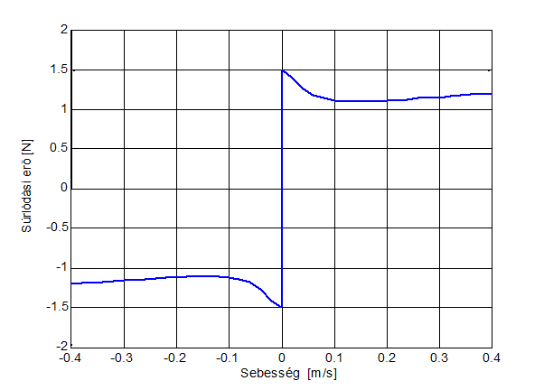
Figure 8-10 shows the steady state friction curve (i.e. Stribeck curve), which have been used for all the cases except the Karnopp model. However there, the value of FC, Fv and Fs were selected similar to that of the steady-state curve.
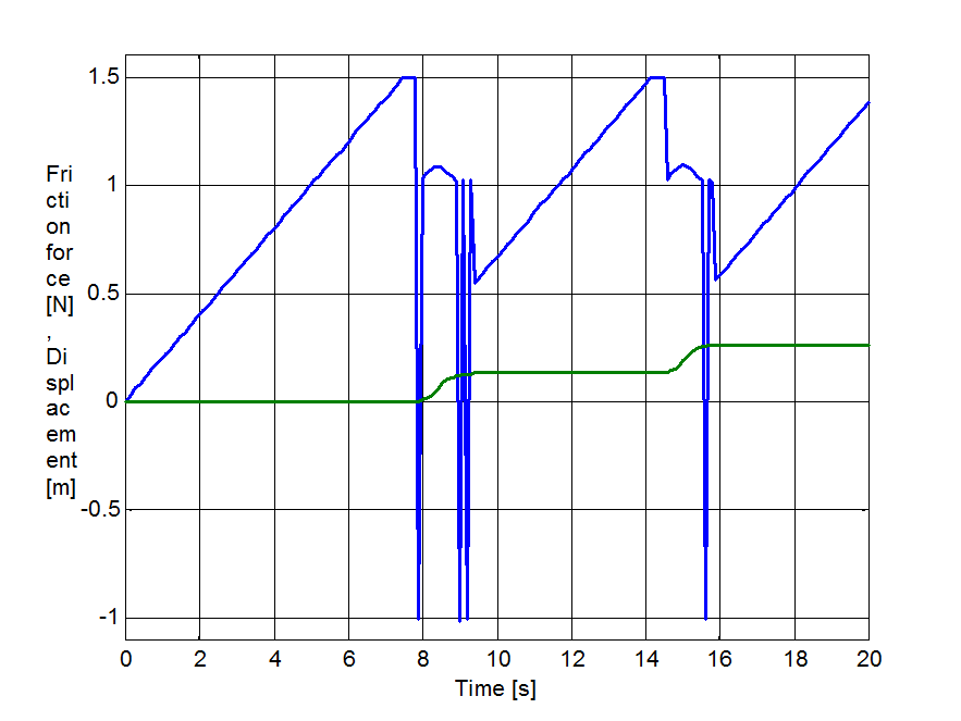
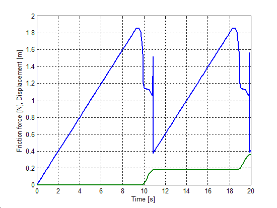
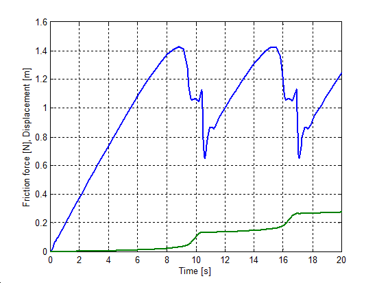
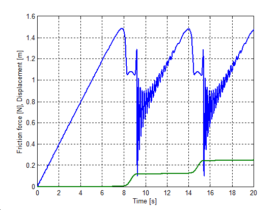
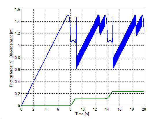
8.6.1. Stick-slip motion
A single unitary mass with friction was pulled by a spring to simulate stick-slip motion. The spring free end was moving with a constant speed. Both the speed and the stiffness of the spring was selected on such a way that stick-slip motion occurred (vspring = 0.02 m/s, kspring = 0.1 N/m). These values were the same in case of all models.
The simulation results are shown by figures from Figure 811 to Figure 815. The upper curve is the force, while the lower one is the displacement as a function of time.
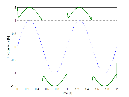
Both the cases of the seven parameter, Karnopp and LuGre models we get a smooth curve. The Karnopp model does not contain time lag, thus the system responds immediately to any change. This is why the force changes over into negative value when the motion begins.
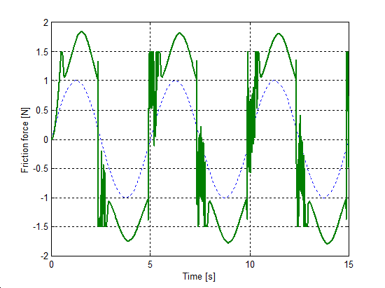
Both the modified Dahl and the M2 models show undesirable oscillations superposed on the friction force, when the mass gets stuck. However, we have to remark that the original source [33] shows a smooth curve for the M2 model. Probably that can be achieved with special parameterization.
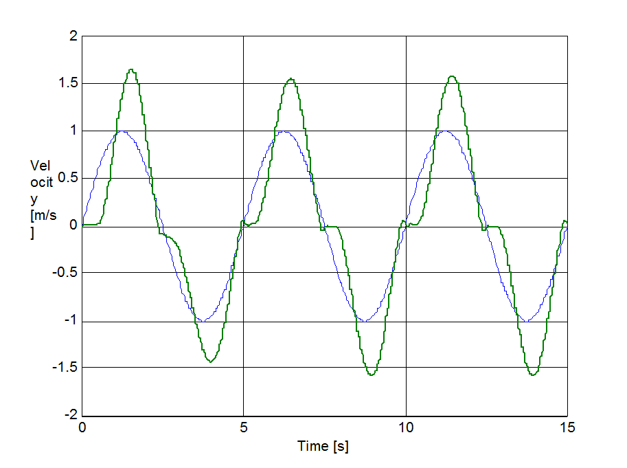
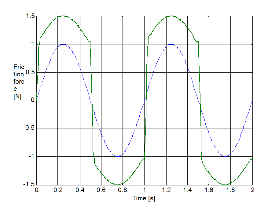
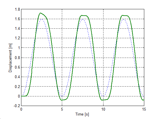
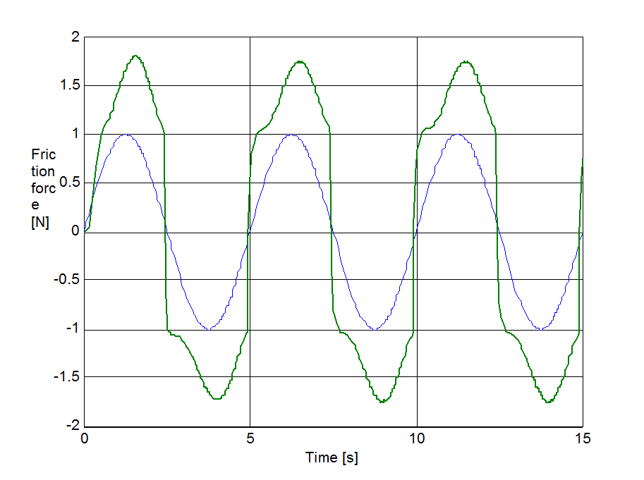
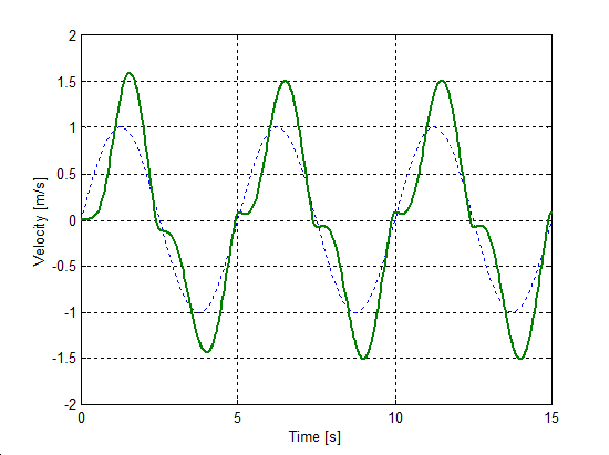
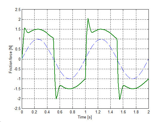
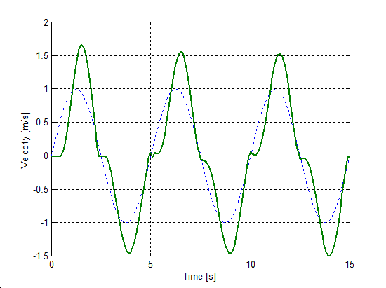
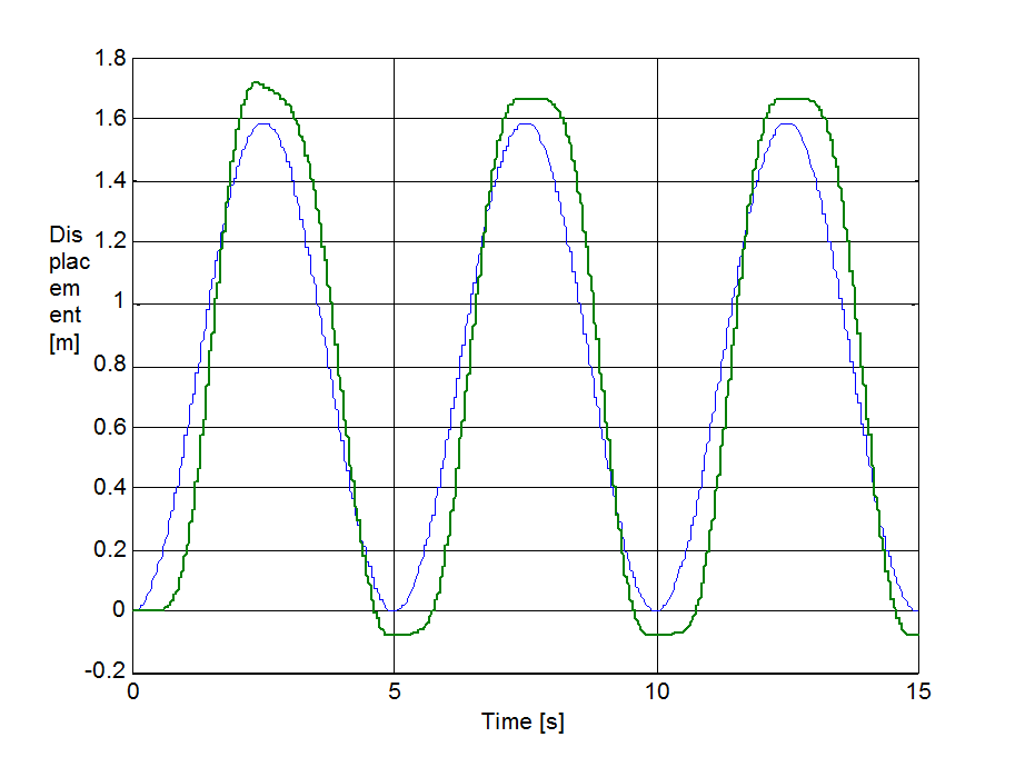
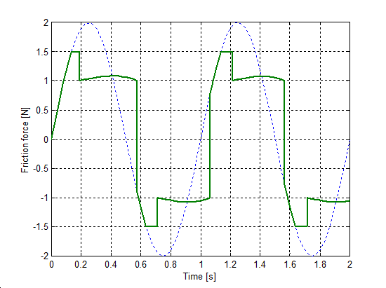
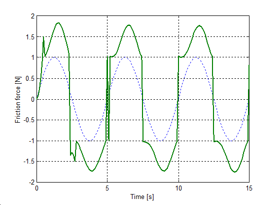
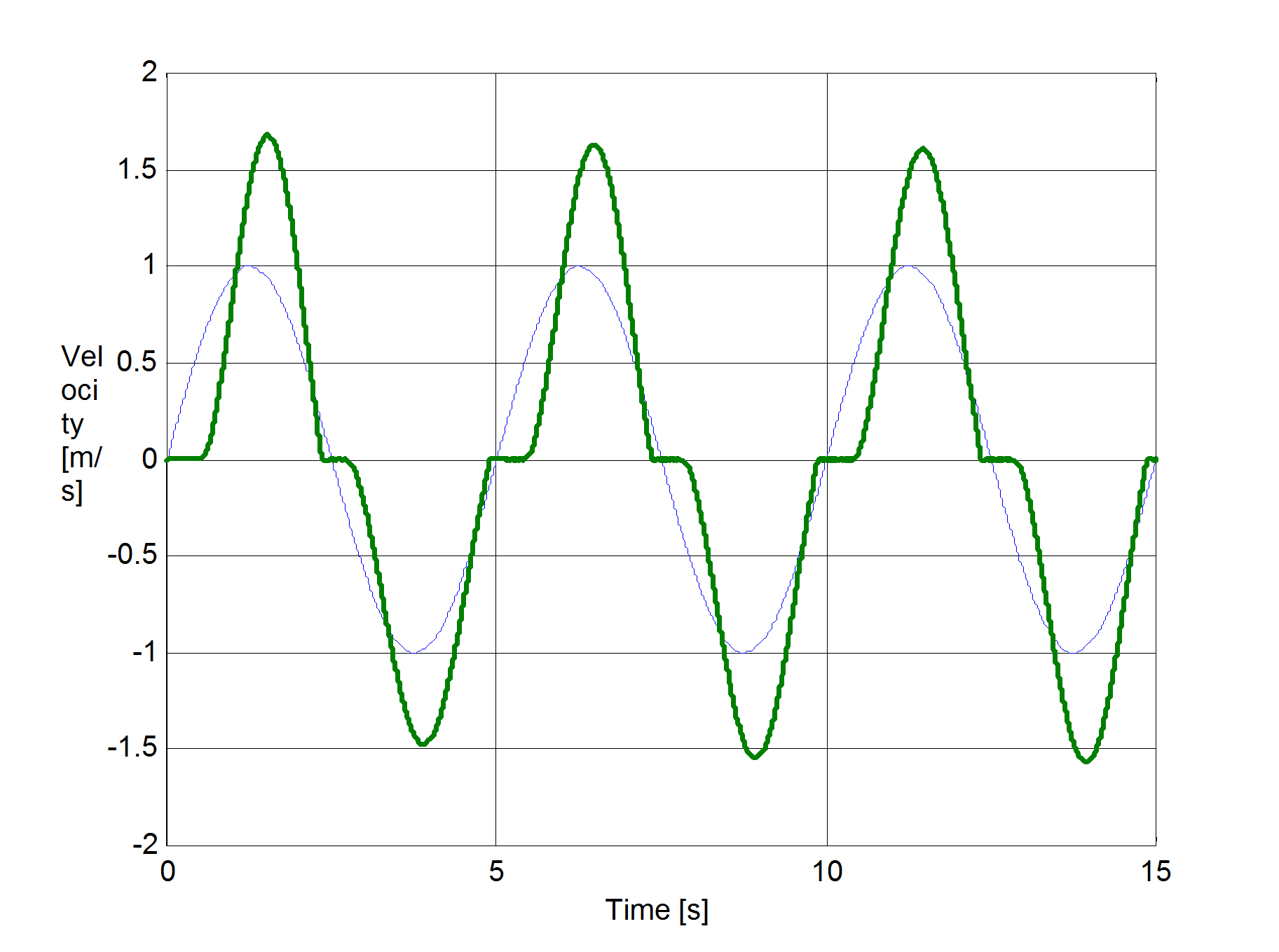
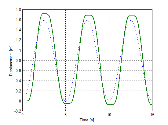
8.6.2. Zero velocity crossing
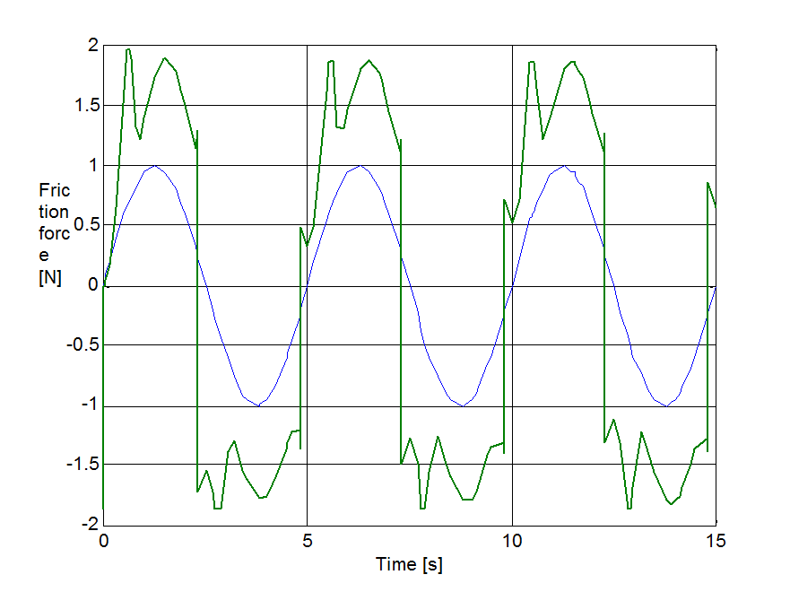
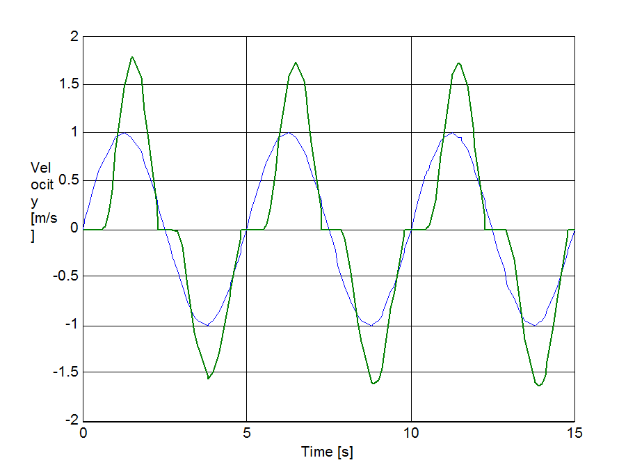
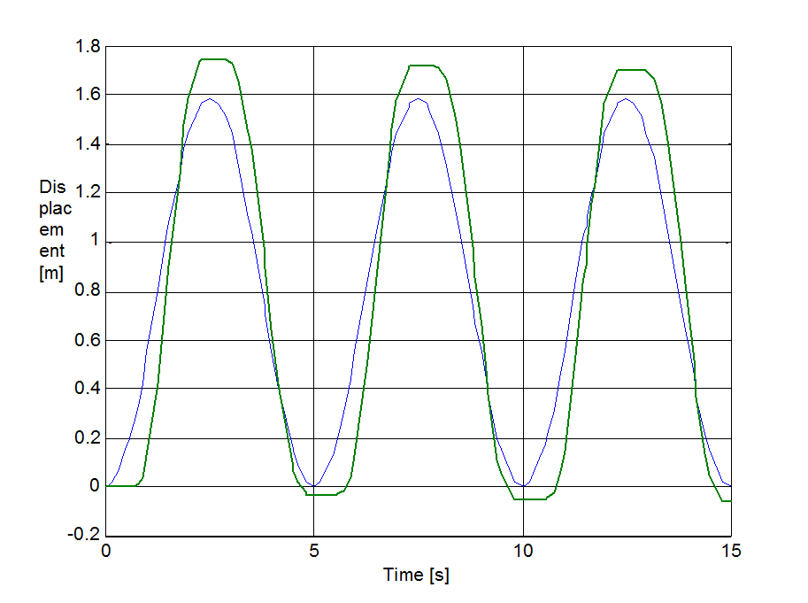
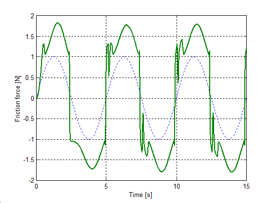
The same set up as of stick-slip was used for velocity reversals testing. The free end of the spring was pulled by a velocity changed as Asin(t), where A = 1 m/s. The simulation results plotted against time are in Figure 8-16 trough Figure 8-35 for friction force, velocity, displacement and spring force for each of the five models respectively. The thin dashed line shows the exciting velocity for all cases, except for displacement, where it is the displacement of the free spring end.
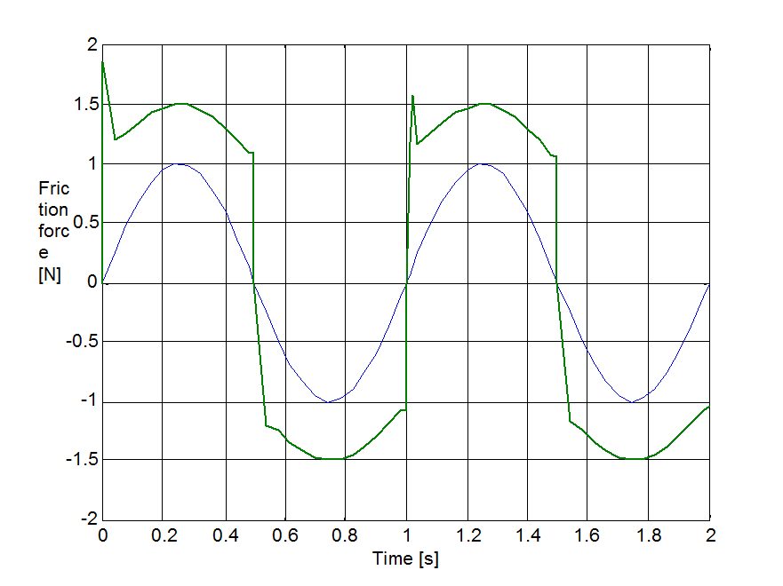

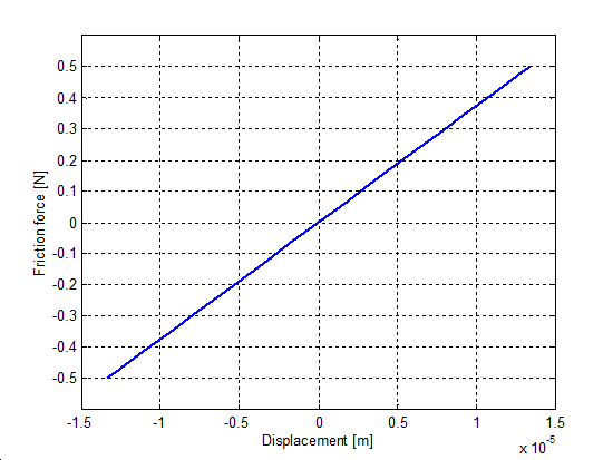
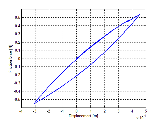
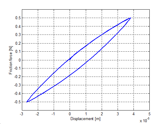
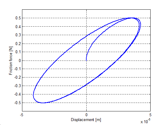
8.6.3. Spring-like stiction behavior
At zero velocities, for force excitation it is desirable that the models show the behavior of a non-linear spring. To simulate this environment a small force, less than the breakaway level was applied with the same magnitude (F = 0.5 N) in each case. The load and unload cycles were ensured by a sinus function with the given amplitude applied on the unitary mass. The resulting presliding displacement curves are in Figure 8-36–Figure 8-39. Note, that the Karnopp friction model does not contain this feature.
Unlike other models, the seven-parameters model does not show any hysteresis. The reason for that, is the seven-parameter model employs a linear spring element for modeling the Dahl effect. It is interesting to note, that the M2 model reaches its steady state only after the first cycle.