Chapter 6. Trajectory execution layer
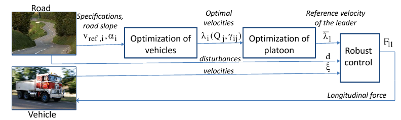
The algorithms presented in the previous section compute the vehicle actions to be carried out in order to achieve the required automation task according to all inputs (automation level, driver automation level request, set of trajectories, relevant detected targets, vehicle positioning, trajectory & state limits, vehicle state). The outputs of this function are primarily the trajectory and the speed constraints. This trajectory has to be realized by a control system considering the fuel economy, the speed constraints and vehicle parameters.
Another task of the trajectory execution layer is the execution of the calculated control commands (motion vector) and to provide feedback about the actual status. The motion vector contains the selected trajectory that has to be followed including the desired longitudinal and lateral movement of the vehicle.
The execution of the motion vector is distributed among the intelligent actuators of the vehicle. The task distribution and the harmonization of the intelligent actuators are carried out by the integrated vehicle (powertrain) controller.
6.1. Longitudinal control
The main task of the longitudinal control is the calculation and execution of an optimal speed profile. It is basically a speed control (cruise control) which tries to hold speed set-point given by the driver, but it could be extended by distance control (ACC) and the road inclinations in front of the vehicle. This control method and the extension to a platoon is detailed in the following subsections.
6.1.1. Design of speed profile
The purpose is to design speed trajectory, with which the longitudinal energy, thus fuel requirement can be reduced. If the inclination of the road and the speed limits are assumed to be known, the speed trajectory can be designed. By choosing the speed fitting in these factors the number of unnecessary accelerations and brakes can be reduced.
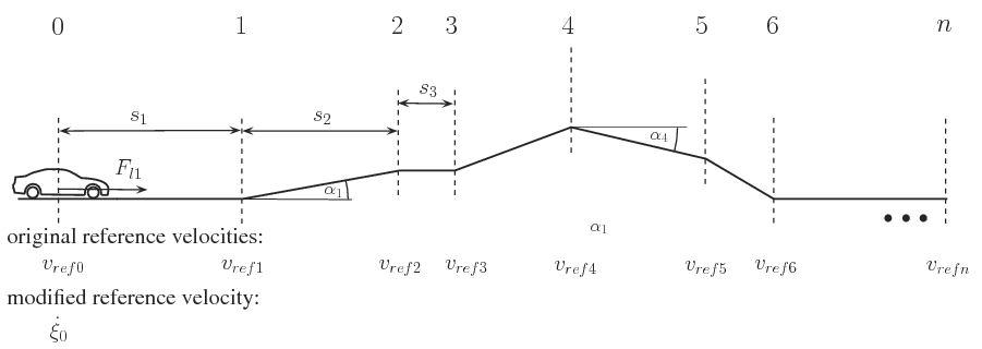
The road ahead of the vehicle is divided into several sections and reference speeds are selected for them, see Figure 87. The rates of the inclinations of the road and those of the speed limits are assumed to be known at the endpoints of each section. The knowledge of the road slopes is a necessary assumption for the calculation of the velocity signal. In practice the slope can be obtained in two ways: either a contour map which contains the level lines is used, or an estimation method is applied. In the former case a map used in other navigation tasks can be extended with slope information. Several methods have been proposed for slope estimation. They use cameras, laser/inertial profilometers, differential GPS or a GPS/INS systems, see [72], [73], [74]. An estimation method based on a vehicle model and Kalman filters was proposed by [75].
The simplified model of the longitudinal dynamics of the vehicle is shown in Figure 88. The longitudinal movement of the vehicle is influenced by the traction force  as the control signal and disturbances
  . Several longitudinal disturbances influence the movement of the vehicle. The rolling resistance is modeled by an empiric form
  where
where  is the vertical load of the wheel,
  and
and  are empirical parameters depending on tyre and road conditions and
  is the velocity of the vehicle, see GOTOBUTTON GrindEQbibitem24 . The aerodynamic force is formulated as
  where
where  is the drag coefficient,
  is the density of air,
  is the reference area,
  is the velocity of vehicle relative to the air. In case of a lull
  , which is assumed in the paper. The longitudinal component of the weighting force is
  , where m is the mass of the vehicle and
  is the angle of the slope. The acceleration of the vehicle is the following:
  , where
  is the mass of the vehicle,
  is the position of the vehicle, and
  are the traction force and the disturbance force (
 ), respectively.
Although between the points may be acceleration and declaration an average speed is used. Thus, the rate of accelerations of the vehicle is considered to be constant between these points. In this case the movement of the vehicle using simple kinematic equations is:  , where
  is the velocity of vehicle at the initial point,
  is the velocity of vehicle at the first point and
  is the distance between these points. Thus the velocity of the first section point is the following:
  . The velocity of the first section point
  is defined as the reference velocity
  . This relationship also applies to the next road section:
  . It is important to emphasize that the longitudinal force
  is known only the first section. Moreover, the longitudinal forces
  are not known during the traveling in the first section. Therefore at the calculation of the control force it is assumed that additional longitudinal forces will not act on the vehicle, i.e., the longitudinal forces
  will not affect the next sections. At the same time the disturbances from road slope are known ahead. Similarly, the velocity of the vehicle can be formalized in the next
  section points. Using this principle a velocity-chain, which contains the required velocities along the way of the vehicle, is constructed. At the calculation of the control force it is assumed that additional longitudinal forces
  will not affect the next sections. The velocities of vehicle are described at each section point of the road by using similar expressions to GOTOBUTTON GrindEQequation22 . The velocity of the
  section point is the following:
 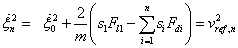 . It is also an important goal to track the momentary value of the velocity. It can also be considered in the following equation:
The  disturbance force can be divided in two parts: the first part is the force resistance from road slope
  , while the second part
  contains all of the other resistances such as rolling resistance, aerodynamic forces etc. We assume that
  is known while
  is unknown.
 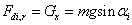 depends on the mass of the vehicle and the angle of the slope
  . When the control force
  is calculated, only
  influences the vehicle of all of the unmeasured disturbances. In the control design the effects of the unmeasured disturbances
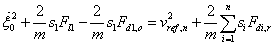
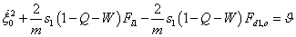
  are ignored. The consequence of this assumption is that the model does not contain all the information about the road disturbances, therefore it is necessary to design a robust speed controller. This controller can ignore the undesirable effects. Consequently, the equations of the vehicle at the section points are calculated in the following way:
|
|
(1) |

|
|
(2) |
|
|
(3) |

|
|
(4) |
The vehicle travels in traffic and it may happen that the vehicle is overtaken. Because of the risk of collision it is necessary to consider the preceding velocity on the lane:
|
|
(5) |

The number of the segments is important. For example in the case of flat roads it is enough to use relatively few section points because the slopes of the sections do not change abruptly. In the case of undulating roads it is necessary to use relatively large number of section points and shorter sections, because it is assumed in the algorithm that the acceleration of the vehicle is constant between the section points. Thus, the road ahead of the vehicle is divided unevenly, which is consistent with the topography of the road.
In the following step weights  are applied to reference speeds. An additional weight
  is applied to the momentary speed. An additional weight
  is applied to the leader speed. While the weights
  represent the rate of the road conditions, weight
  has an essential role: it determines the tracking requirement of the current reference velocity
  . By increasing
  the momentary velocity becomes more important while road conditions become less important. Similarly, by increasing
  the road conditions and the momentary velocity become negligible. The weights should sum up to one, i.e.
  .
.
Weights have an important role in control design. By making an appropriate selection of the weights the importance of the road condition is taken into consideration. For example when  and
and  the control exercise is simplified to a cruise control problem without any road conditions. When equivalent weights are used the road conditions are considered with the same importance, i.e.,
  and
and  . When
  and
and 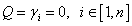 only the tracking of the preceding vehicle is carried out. The optimal determination of the weights has an important role, i.e., to achieve a balance between the current velocity and the effect of the road slope. Consequently, a balance between the velocity and the economy parameters of the vehicle is formalized.
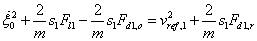
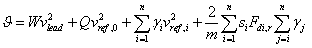
By summarizing the above equations the following formula is yielded:
|
|
(6) |
where the value  depends on the road slopes, the reference velocities and the weights
|
|
(7) |
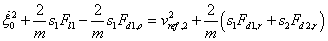
In the final step a control-oriented vehicle model, in which reference velocities and weights are taken into consideration, is constructed. The momentary acceleration of the vehicle is expressed in the following way: 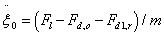 where
where  . Equation (6) is rearranged:
|
|
(8) |

where the parameter 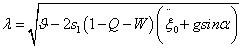 is calculated based on the designed
  . Consequently, the road conditions can be considered by speed tracking. The momentary velocity of vehicle
  should be equal to parameter
  , which contains the road information. The calculation of
  requires the measurement of the longitudinal acceleration
  .
.
6.1.2. Optimization of the vehicle cruise control
In the following step the task is to find an optimal selection of the weights in such a way that both the minimization of control force and the traveling time are taken into consideration. Equation (6) shows that  depends only on the weights in the following way:
|
|
(9) |

Since  depends on the weight
  , therefore
  depends on the weights
  and
and  . The longitudinal control force must be minimized, i.e.,
  . Instead, in practice the
  optimization is used because of the simpler numerical computation. Simultaneously, the difference between momentary velocity and modified velocity must be minimized, i.e.,
The two optimization criteria lead to different optimal solutions. In the first criterion the road inclinations and speed limits are taken into consideration by using appropriately chosen weights  . At the same time the second criterion is optimal if the information is ignored. In the latter case the weights are noted by
  . The first criterion is met by the transformation of the quadratic form into the linear programming using the simplex algorithm. It leads to the following form:
  with the following constrains
  and
and  . This task is nonlinear because of the weights. The optimization task is solved by a linear programming method, such as the simplex algorithm.
The second criterion must also be taken into consideration. The optimal solution can be determined in a relatively easy way since the vehicle tracks the predefined velocity if the road conditions are not considered. Consequently, the optimal solution is achieved by selecting the weights in the following way:  and
and  .
.
In the proposed method two further performance weights, i.e.,  and
and  , are introduced. The performance weight
  (
( ) is related to the importance of the minimization of the longitudinal control force
  while the performance weight
  is related to the minimization of
  . There is a constraint according to the performance weights
  . Thus the performance weights, which guarantee balance between optimizations tasks, are calculated in the following expressions:
|
|
(10) |
 , i=1,n(11)
Based on the calculated performance weights the speed can be predicted.
The tracking of the preceding vehicle is necessary to avoid a collision, therefore  is not reduced. If the preceding vehicle accelerates, the tracking vehicle must accelerate as well. As the velocity increases so does the braking distance, therefore the following vehicle strictly tracks the velocity of the preceding vehicle. On the other hand it is necessary to prevent the velocity of the vehicle from increasing above the official speed limit. Therefore the tracked velocity of the preceding vehicle is limited by the maximum speed. If the preceding vehicle accelerates and exceeds the speed limit the following vehicle may fall behind.
Remark 3.1 Look-ahead control considering efficiency and safe cornering
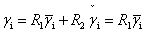
The maximum cornering velocity for each section can be calculated in advance knowing the designed path of the vehicle. If the speed limit  at section point
  exceeds the safe cornering velocity then the speed limit
  is substituted with the smallest value concerning skidding or rollover, i.e.,
|
|
(12) |
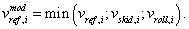
6.1.3. Implementation of the velocity design
The control system can be realized in three steps as Figure 89 shows. The aim of the first step is the computation of the reference velocity. The results of this computation are the weights and the modified velocity which must be tracked by the vehicle. In the second step the longitudinal control force of the vehicle ( ) is designed. The role of the high-level controller is to calculate this required longitudinal force. In third step the real physical inputs of the system, such as the throttle, the gear position and the brake pressure are generated by the low-level controller.
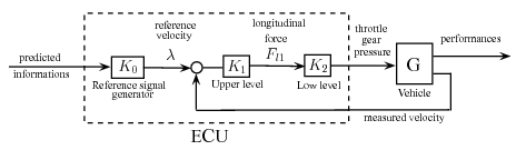
In the proposed method the steps are separated from each other. The reference velocity signal generator can be added to the upper-lower Adaptive Cruise Control (ACC) system. It is possible to design a reference signal generator unit almost individually, and to attach it to the ACC system. Thus the reference signal unit can be designed and produced independently from automobile suppliers, only a few vehicle data are needed. The independent implementation possibility is an important advantage in practice. The high-level controller calculates positive and negative forces as well, therefore the driving and braking systems are also actuated. Figure 90 shows the architecture of the low-level controller.
The engine is controlled by the throttle, which could be a butterfly gate or a quantity of injected fuel. The engine-management system and the fuel-injection system have their own controllers, thus in the realization of the low-level controller only the torque-rev-load characteristics of the engine are necessary. In this case the rev of the engine is measured, the required torque is computed from the longitudinal force of the high-level controller, thus the throttle is determined by an interpolation step using a look-up table. The position of the automatic transmission is determined by logic functions, thus it depends on the fuel consumption and the maximum rev of the engine. The pressures on the cylinders of the wheels increase during braking. At normal traveling the ABS actuation is not necessary, in case of an emergency the optimal driving is overwritten by the safety requirements. The necessary braking pressure for the required braking force is computed from the ratios of the hydraulic/pneumatic parts.
In the simulation example a transportational route with real data is analyzed. The terrain characteristics and geographical information are those of the M1 Hungarian highway between Tatabánya and Budapest in a  -
- -long section. In the simulation a typical F-Class truck travels along the
  route. The mass of the 6--gear truck is
  and its engine power is
  (
( ). The regulated maximal velocity is
  , but the road section contains other speed limits (e.g.
  or
or  ), and the road section also contains hilly parts. Thus, it is an acceptable route for the analysis of road conditions, i.e., inclinations and speed limits. Publicly accessible up-to-date geographical/navigational databases and visualisation programs, such as Google Earth and Google Maps, are used for the experiment.
|
|
|
|
|
|
|
|
|
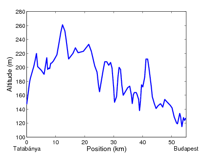
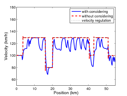
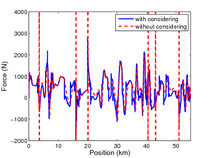
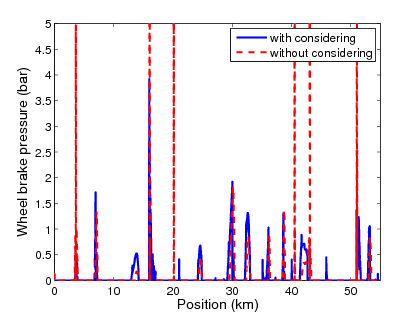
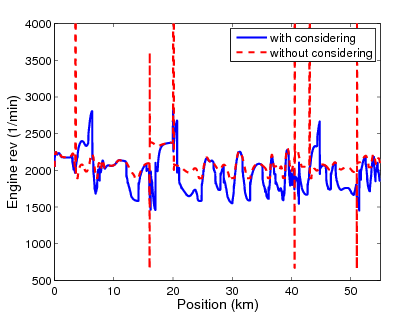
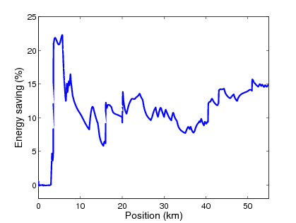
Figure 91: Real data motorway simulation
In this example two different controllers are compared. The first is the proposed controller, which considers the road conditions such as inclinations and speed limits and is illustrated by solid line in the figures, while the second controller is a conventional ACC system, which ignores this information and is illustrated by dashed line. Figure 91 shows the time responses of the simulation.
Figure 91(a) shows that the motorway contains several uphill and downhill sections. Figure 91(b) shows the velocity of the vehicle with speed limits in both cases. The conventional ACC system tracks the predefined speed limits as accurately as possible and the tracking error is minimal. In the proposed method the speed is determined by the speed limits and simultaneously it takes the road inclinations into consideration according to the optimal requirement. Figure 91(c) shows the required longitudinal force. The high-precision tracking of the predefined velocities in the conventional ACC system often requires extremely high forces with abrupt changes in the signals. As a result of the road conditions less energy is required during the journey in the proposed control method, see Figure 91(f). The proposed method requires smaller energy ( ) than the conventional method (
 ), and the energy saving is
  , which is
  . The fuel consumption can also be calculated by using the following approximation:
 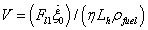 where
where  is the efficiency of the driveline system,
 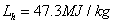 is the heat of combustion and
  is the density of petrol. The fuel consumption of the conventional system is
  while that of the proposed method is
  , which results in
  reduction in fuel consumption in the analyzed
  length section.
Remark 3.2 Speed control based on the preceding vehicle
In addition to the consideration of road conditions it is also important to consider the traffic environment. It means that the preceding vehicle must be considered in the reference speed design because of the risk of collision. Thus, all of the kinetic energy of the vehicle is dissipated by friction. This estimation of the safe stopping distance may be conservative in a normal traffic situation, where the preceding vehicle also brakes, therefore the distance between the vehicles may be reduced. In this paper the safe stopping distance between the vehicles is determined according to the 91/422/EEC, 71/320/EEC UN and EU directives (in case of  vehicle category, the velocity in
  ):
):  . It is also necessary to consider that without the preceding vehicle the consideration of safe stopping distance is neither possible nor necessary. The consideration of the preceding vehicle is determined by
  . The following example analyses the incidence when another vehicle overtakes the vehicle with an adaptive control proposed in the paper or the vehicle catches up with a preceding vehicle.
In the simulation example, the preceding vehicle is slower, however, in the second part its velocity is higher than that of the follower vehicle. Furthermore, in the example the preceding vehicle also exceeds the official speed limit ( ). Figure 92(a) and Figure 92(b) show that in the first part of the simulation the follower vehicle approaches the preceding vehicle taking the braking distance into consideration, while in the second part the follower vehicle avoids exceeding the speed limit and falls behind. This velocity control is achieved by using the value of
  as it is shown in Figure 92(d). In the first part of the simulation the weight is increased by the risk incident while in the second part it is reduced by the increasing distance. The solution requires radar information, which is available in a conventional adaptive cruise control vehicle. This simulation example shows that the designed control system is able adapt to external circumstances.
|
|
|
|
|
|
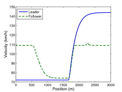
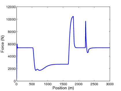
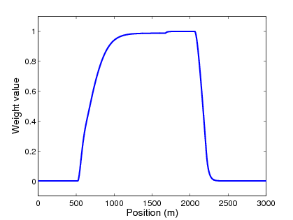
Figure 92: Adaptive control systems with a preceding vehicle
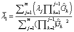
6.1.4. Extension of the method to a platoon
The main idea behind the design is that each vehicle in the platoon is able to calculate its speed independently of the other vehicles. Since traveling in a platoon requires the same speed, the optimal speed must be modified according to the other vehicles. In the platoon, the speed of the leader vehicle determines the speed of all the vehicles. The goal is to determine the common speed at which the speeds of the members are as close as possible to their own optimal speed. In the case of a platoon each vehicle has its own optimal reference speed  . Moreover, speeds of the vehicles are not independent of each other, because the speed of the leader
  influences the speed of every member of platoon
  . The goal is to find an optimal reference speed for the leader
  .
.
It is important to note that there is an interaction between the speeds of the vehicles in a platoon. If a preceding vehicle changes its speed, the follower vehicles will modify their speeds and track the motion of the preceding vehicle within a short time. The members of the platoon are not independent of the leader, therefore it is necessary to formulate the relationship between the speed of the  platoon member
  and the leader and the preceding vehicles. It is formulated with a transfer function with its input and output. The output
  contains the information, i.e., the position, speed and acceleration of the vehicle, which is sent to the follower vehicles. The input
  contains the position, speed, the acceleration of the preceding vehicle and the leader. The transfer function between
  and
and  is
is  with the controller of the
  vehicle
  and its longitudinal dynamics
  . Similarly, the effect of the leader and the preceding vehicles on the
  platoon member is formulated:
  , where
  , which finally leads to
  . Consequently, the speed of the
  vehicle is determined by the next formula:
 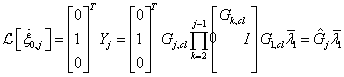 . The value of
  is used for the computation of the optimal reference speed of the platoon
  .
.
Finally the required reference speed of the leader vehicle  is designed. The aim of the design is that the generated speeds of all the vehicles
  are as close to as their modified reference speed
  as possible:
|
|
(13) |
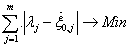
Since the speed of the  vehicle is formulated as
  , the following optimization form is used:
 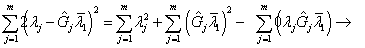 , where
  . It can be stated that in GOTOBUTTON GrindEQequation48 the only unknown variable is
  . The optimization leads to the following equation:
 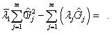 The solution of the optimization problem can be achieved. The deduction of the optimization of
  is as follows:
|
|
(14) |
It means that the leader vehicle must track the required reference speed  .
.
6.2. Lateral control
6.2.1. Design of trajectory
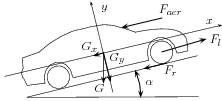
Government transportation agencies have been evaluating several studies in the field of highway road planning in respect to horizontal curve design. Road design manuals determine a minimum curve radius for a predefined velocity, road superelevation and adhesion coefficient, see [76], [77]. The calculation is based on assuming the vehicle to move on a circular path, where the vehicle is subject to centrifugal force that acts away from the center of the curve as illustrated in Figure 94, see [78]. The slip angle  is assumed to be small enough for the lateral force to point along the path radius, and the longitudinal acceleration is also small enough not to degrade the lateral friction of the vehicle considerably.
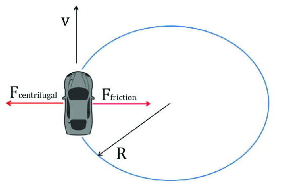
The mass of the vehicle  along with the road superelevation (cross slope)
  and the side friction between the tire and the road surface
  counterbalance the centrifugal force. Assuming that there is the same
  at each wheel of the vehicle the sum of the lateral forces is:
 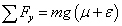 , where
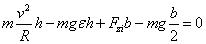
  is the gravitational constant. At cornering the dynamics of vehicle is described by the equilibrium of the two forces:
  , where
  is the radius of the curve. Assuming that the road geometry is known by on-board devices such as GPS, it is possible to calculate a safe cornering velocity.
The following relationship holds for the maximum safe cornering velocity regarding the danger of skidding out of the corner:
|
|
(15) |
(15) is also used in crash reconstruction and is referred to as the Critical Speed Formula (CSF), see [79], [80]. In the so-called yaw mark method the critical speed of the vehicle is determined by using the calculated radius of the vehicle path from the tire skid marks left on the road.
Note that in the calculation of the safe cornering velocity the value of the side friction factor  plays a major role. This factor depends on the quality and the texture of the road, the weather conditions and the velocity of the vehicle and several other factors. The estimation of
  has been presented by several important papers, see e.g. [81], [82], [83]. However, these estimations are based on instant measurements, thus they are not valid for look-ahead control design, where the friction of future road sections should be estimated.
In road design handbooks the value of the friction factor is given in look-up tables as a function of the design speed, and it is limited in order to determine a comfortable side friction for the passengers of the vehicle. For the calculation of safe cornering velocity these friction values give a very conservative result.
A method to evaluate side friction in horizontal curves using supply-demand concepts has been presented by [84]. Here the side friction has an exponential relation with the design speed as follows:
|
|
(16) |
where  and
and  are constant values depending on the texture of the pavement. Note that
  is the estimated reference friction at a measurement speed of
  . Thus, by using (15) and (16) the maximum safe cornering speed can be determined on a given road surface along with the side friction factor, as it is illustrated inFigure 95. The intersections of the supply and demand curves give the safe cornering velocities and the corresponding maximum side frictions. Note that whereas the friction supply only depends on the velocity of the vehicle, the friction demand is a function of the velocity and the curve radius as well.
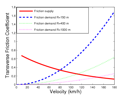
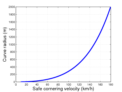
The relationship between the curve radius and safe cornering velocity can be observed in Figure 5. The data points of the diagram are given by the intersections of the supply and demand curves. It shows that the safe cornering velocity increases with the curve radius. However, the relationship is not linear, i.e by increasing an already big cornering radius results in only moderated growth of the safe cornering velocity.
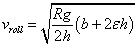
Rollover danger estimation and prevention control methods have already been studied by several authors, see [85], [86], [87]. A quasi-static analysis of maximal safe cornering velocity regarding the danger of rollover has been presented by [88]. Assuming a rigid vehicle and using small angle approximation for superelevation ( ,
,  ), a moment equation can be written for the outside tires of the vehicle during cornering as follows:
|
|
(17) |
where  is the height of the center of gravity,
  is the track width,
  is the load of the inside wheel at cornering.
The vehicle stability limit occurs at the point when the load  reaches zero, which means the vehicle can no longer maintain equilibrium in the roll plane. Thus by reorganizing (17) and substituting
  the rollover threshold is given as follows:
|
|
(18) |
Thus, to ensure safe cornering of the vehicle in a cornering maneuver without the danger of skidding or rollover, the velocity of the vehicle has to chosen to meet the two constraints defined by (15) and (16).
6.2.2. Road curve radius calculation
Another important task is to calculate the radius of curves ahead of the vehicle in order to define the safe cornering velocities in advance. The road ahead of the vehicle can be divided into  number of sections. The goal is to calculate the curve radius at each
  section points ahead of the vehicle to determine the safe cornering velocities corresponding to the curve radius.
The calculation of the cornering radius  ,
,  is as follows. It is assumed that the global trajectory coordinates
  and
and  of the vehicle path are known. Considering a sufficiently small distance the trajectory of the vehicle around a section point can be regarded as an arc, as it is shown in Figure 97. The arc can be divided into
  data points.
The length of the arc can be approximated by summing up the distances between data points:  These distances are calculated as:
 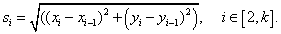 The length of the chord
  is calculated as follows:
  Knowing the length
  and
and  ,
,  it is possible to calculate a reasonable estimation of the curve radius
  . Note that the length of the arc must be chosen carefully. A too short section with fewer data points may give an unacceptable approximation of the radius. On the other hand a too big distance can be inappropriate as well, since then the section may not be approximated by a single arc. The number of data points selected is also important, and by increasing the number
  , the accuracy of the following calculation can be enhanced. The angle of the arc
  is as follows
  . The length of the chord
  is also expressed as a function of the radius:
  . Expressing the radius
  the following equation is derived:
|
|
(19) |
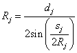
This expression can be transformed by introducing  and using the Taylor series for the approximation of the
  function, i.e.,
  . Then the following expression is gained for the radius:
|
|
(20) |
The curve radius  ,
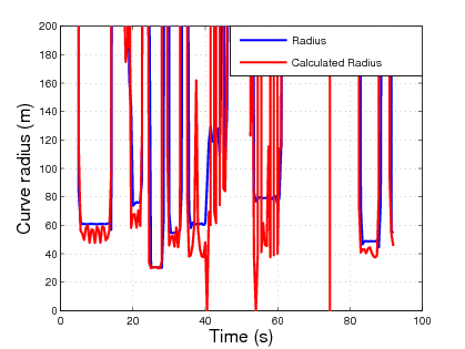
,  can be calculated at each section point ahead of the vehicle path. The calculation method is validated through the CarSim simulation environment. Here, the vehicle follows the desired path while the curve radius is being measured and at the same time the calculation method is running giving a close approximation of the real value. The comparison of the real and the calculated radius is shown in Figure 98.
By calculating the radius of the curve using (20) the safe cornering velocity of the vehicle can be determined by using (15) and (18). This velocity can be considered as the maximum velocity that the vehicle is capable of in a corner without the danger of slipping and leaving the track or rolling over. It is important to state that in severe weather conditions this safe velocity may be smaller than that of the speed limit, thus the consideration of the maximum safety velocity in the cruise control design is essential.